You have seen in previous chapters how sounds are generally composed of multiple frequency components. Sometimes it’s desirable to increase the level of some frequencies or decrease others. To deal with frequencies, or bands of frequencies, selectively, we have to separate them out. This is done by means of filters. The frequency processing tools in the following sections are all implemented with one type of filter or another.

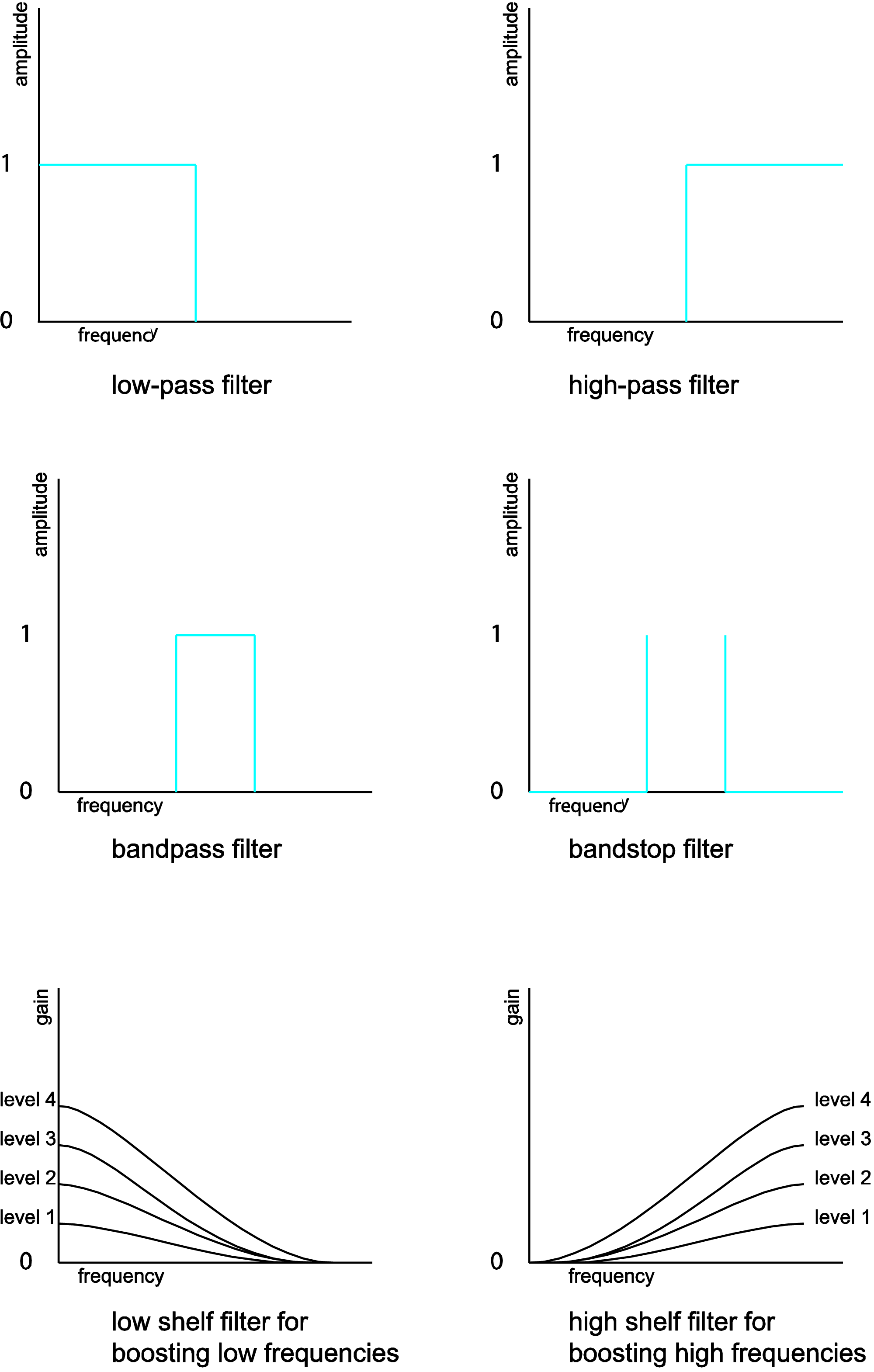
There are a number of ways to categorize filters. If we classify them according to what frequencies they attenuate, then we have these types of band filters:

• low-pass filter – retains only frequencies below a given threshold
• high-pass filter – retains only frequencies above a given threshold
• bandpass filter – retains only frequencies within a given frequency band
• bandstop filter – eliminates frequencies within a given frequency band
• comb filter – attenuates frequencies in a manner that, when graphed in the frequency domain, has a “comb” shape. That is, multiples of some fundamental frequency are attenuated across the audible spectrum
• peaking filter – boosts or attenuates frequencies in a band
• shelving filters
  • low-shelf filter – boosts or attenuates low frequencies
  • high-shelf filter – boosts or attenuates high frequencies

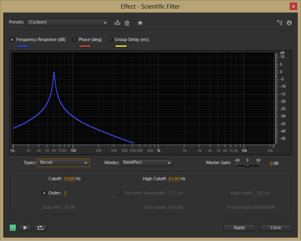
Filters that have a known mathematical basis for their frequency response graphs and whose behavior is therefore predictable at a finer level of detail are sometimes called scientific filters. This is the term Adobe Audition uses for Bessel, Butterworth, Chebyshev, and elliptical filters. The Bessel filter’s frequency response graph is shown in Figure 7.2

If we classify filters according to the way in which they are designed and implemented, then we have these types:

• IIR filters – infinite impulse response filters
• FIR filters – finite impulse response filters

Adobe Audition uses FIR filters for its graphic equalizer but IIR filters for its parametric equalizers (described below.) This is because FIR filters give more consistent phase response, while IIR filters give better control over the cutoff points between attenuated and non-attenuated frequencies. The mathematical and algorithmic differences of FIR and IIR filters are discussed in Section 3. The difference between designing and implementing filters in the time domain vs. the frequency domain is also explained in Section 3.

Convolution filters are a type of FIR filter that can apply reverberation effects so as to mimic an acoustical space. The way this is done is to record a short loud burst of sound in the chosen acoustical space and use the resulting sound samples as a filter on the sound to which you want to apply reverb. This is described in more detail in Section 7.1.6.

Audio equalization, more commonly referred to as EQ, is the process of altering the frequency response of an audio signal. The purpose of equalization is to increase or decrease the amplitude of chosen frequency components in the signal. This is achieved by applying an audio filter.

EQ can be applied in a variety of situations and for a variety of reasons. Sometimes, the frequencies of the original audio signal may have been affected by the physical response of the microphones or loudspeakers, and the audio engineer wishes to adjust for these factors. Other times, the listener or audio engineer might want to boost the low end for a certain effect, “even out” the frequencies of the instruments, or adjust frequencies of a particular instrument to change its timbre, to name just a few of the many possible reasons for applying EQ.

Equalization can be achieved by either hardware or software. Two commonly-used types of equalization tools are graphic and parametric EQs. Within these EQ devices, low-pass, high-pass, bandpass, bandstop, low shelf, high shelf, and peak-notch filters can be applied.

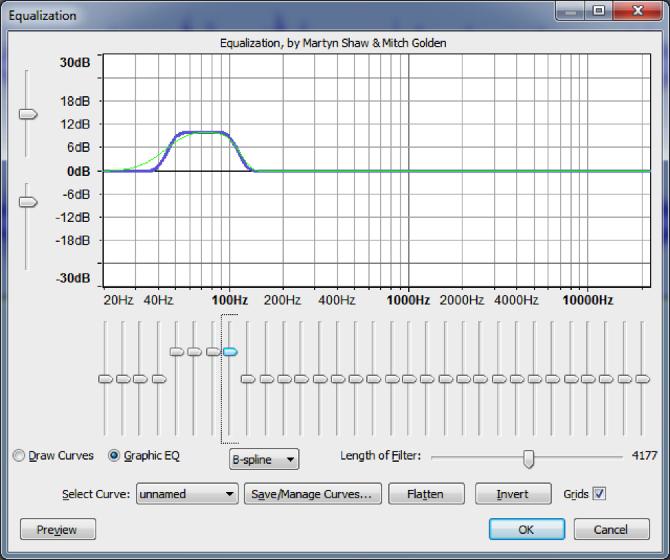
A graphic equalizer is one of the most basic types of EQ. It consists of a number of fixed, individual frequency bands spread out across the audible spectrum, with the ability to adjust the amplitudes of these bands up or down. To match our non-linear perception of sound, the center frequencies of the bands are spaced logarithmically. A graphic EQ is shown in Figure 7.3. This equalizer has 31 frequency bands, with center frequencies at 20 Hz, 25, Hz, 31 Hz, 40 Hz, 50 Hz, 63 Hz, 80 Hz, and so forth in a logarithmic progression up to 20 kHz. Each of these bands can be raised or lowered in amplitude individually to achieve an overall EQ shape.

While graphic equalizers are fairly simple to understand, they are not very efficient to use since they often require that you manipulate several controls to accomplish a single EQ effect. In an analog graphic EQ, each slider represents a separate filter circuit that also introduces noise and manipulates phase independently of the other filters. These problems have given graphic equalizers a reputation for being noisy and rather messy in their phase response. The interface for a graphic EQ can also be misleading because it gives the impression that you’re being more precise in your frequency processing than you actually are. That single slider for 1000 Hz can affect anywhere from one third of an octave to a full octave of frequencies around the center frequency itself, and consequently each actual filter overlaps neighboring ones in the range of frequencies it affects. In short, graphic EQs are generally not preferred by experienced professionals.

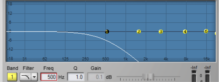
A parametric equalizer, as the name implies, has more parameters than the graphic equalizer, making it more flexible and useful for professional audio engineering. Figure 7.4 shows a parametric equalizer. The different icons on the filter column show the types of filters that can be applied. They are, from top to bottom, peak-notch (also called bell), low-pass, high-pass, low shelf, and high shelf filters. The available parameters vary according to the filter type. This particular filter is applying a low-pass filter on the fourth band and a high-pass filter on the fifth band.

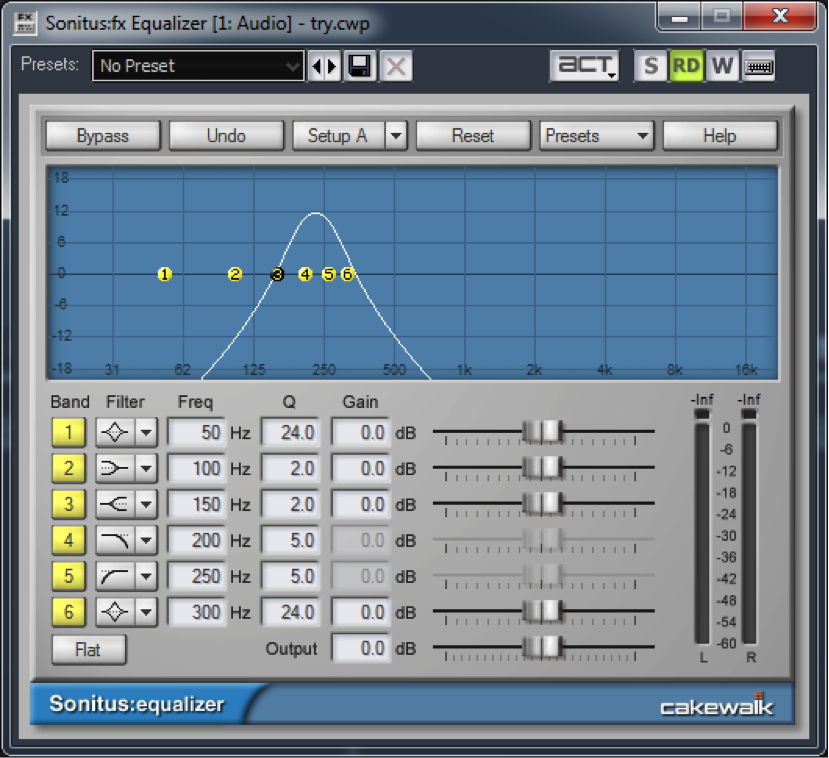
[aside]The term “paragraphic EQ” is used for a combination of a graphic and parametric EQ, with sliders to change amplitudes and parameters that can be set for Q, cutoff frequency, etc.[/aside]

For the peak-notch filter, the frequency parameter corresponds to the center frequency of the band to which the filter is applied. For the low-pass, high-pass, low-shelf, and high-shelf filters, which don’t have an actual “center,” the frequency parameter represents the cut-off frequency. The numbered circles on the frequency response curve correspond to the filter bands. Figure 7.5 shows a low-pass filter in band 1 where the 6 dB down point – the point at which the frequencies are attenuated by 6 dB – is set to 500 Hz.

The gain parameter is the amount by which the corresponding frequency band is boosted or attenuated. The gain cannot be set for low or high-pass filters, as these types of filters are designed to eliminate all frequencies beyond or up to the cut-off frequency.

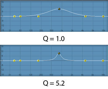
The Q parameter is a measure of the height vs. the width of the frequency response curve. A higher Q value creates a steeper peak in the frequency response curve compared to a lower one, as shown in Figure 7.6.

Some parametric equalizers use a bandwidth parameter instead of Q to control the range of frequencies for a filter. Bandwidth works inversely from Q in that a larger bandwidth represents a larger range of frequencies. The unit of measurement for bandwidth is typically an octave. A bandwidth value of 1 represents a full octave of frequencies between the 6 dB down points of the filter.

cpu'[wpfilebase tag=file id=155 tpl=supplement /]

When you work with sound either live or recorded, the sound is generally captured with the microphone very close to the source of the sound. With the microphone very close, and particularly in an acoustically treated studio with very little reflected sound, it is often desired or even necessary to artificially add a reverberation effect to create a more natural sound, or perhaps to give the sound a special effect. Usually a very dry initial recording is preferred, so that artificial reverberation can be applied more uniformly and with greater control.

There are several methods for adding reverberation. Before the days of digital processing this was accomplished using a reverberation chamber. A reverberation chamber is simply a highly reflective, isolated room with very low background noise. A loudspeaker is placed at one end of the room and a microphone is placed at the other end. The sound is played into the loudspeaker and captured back through the microphone with all the natural reverberation added by the room. This signal is then mixed back into the source signal, making it sound more reverberant. Reverberation chambers vary in size and construction, some larger than others, but even the smallest ones would be too large for a home, much less a portable studio.

Because of the impracticality of reverberation chambers, most artificial reverberation is added to audio signals using digital hardware processors or software plug-ins, commonly called reverb processors. Software digital reverb processors use software algorithms to add an effect that sounds like natural reverberation. These are essentially delay algorithms that create copies of the audio signal that get spread out over time and with varying amplitudes and frequency responses.

A sound that is fed into a reverb processor comes out of that processor with thousands of copies or virtual reflections. As described in Chapter 4, there are three components of a natural reverberant field. A digital reverberation algorithm attempts to mimic these three components.

The first component of the reverberant field is the direct sound. This is the sound that arrives at the listener directly from the sound source without reflecting from any surface. In audio terms, this is known as the dry or unprocessed sound. The dry sound is simply the original, unprocessed signal passed through the reverb processor. The opposite of the dry sound is the wet or processed sound. Most reverb processors include a wet/dry mix that allows you to balance the direct and reverberant sound. Removing all of the dry signal leaves you with a very ambient effect, as if the actual sound source was not in the room at all.

The second component of the reverberant field is the early reflections. Early reflections are sounds that arrive at the listener after reflecting from the first one or two surfaces. The number of early reflections and their spacing vary as a function of the size and shape of the room. The early reflections are the most important factor contributing to the perception of room size. In a larger room, the early reflections take longer to hit a wall and travel to the listener. In a reverberation processor, this parameter is controlled by a pre-delay variable. The longer the pre-delay, the longer time you have between the direct sound and the reflected sound, giving the effect of a larger room. In addition to pre-delay, controls are sometimes available for determining the number of early reflections, their spacing, and their amplitude. The spacing of the early reflections indicates the location of the listener in the room. Early reflections that are spaced tightly together give the effect of a listener who is closer to a side or corner of the room. The amplitude of the early reflections suggests the distance from the wall. On the other hand, low amplitude reflections indicate that the listener is far away from the walls of the room.

The third component of the reverberant field is the reverberant sound. The reverberant sound is made of up all the remaining reflections that have bounced around many surfaces before arriving at the listener. These reflections are so numerous and close together that they are perceived as a continuous sound. Each time the sound reflects off a surface, some of the energy is absorbed. Consequently, the reflected sound is quieter than the sound that arrives at the surface before being reflected. Eventually all the energy is absorbed by the surfaces and the reverberation ceases. Reverberation time is the length of time it takes for the reverberant sound to decay by 60 dB, effectively a level so quiet it ceases to be heard. This is sometimes referred to as the RT60, or also the decay time. A longer decay time indicates a more reflective room.

Because most surfaces absorb high frequencies more efficiently than low frequencies, the frequency response of natural reverberation is typically weighted toward the low frequencies. In reverberation processors, there is usually a parameter for reverberation dampening. This applies a high shelf filter to the reverberant sound that reduces the level of the high frequencies. This dampening variable can suggest to the listener the type of reflective material on the surfaces of the room.

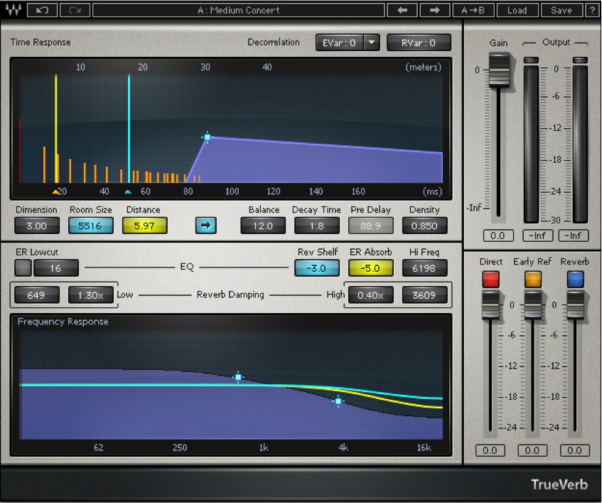
Figure 7.7 shows a popular reverberation plug-in. The three sliders at the bottom right of the window control the balance between the direct, early reflection, and reverberant sound. The other controls adjust the setting for each of these three components of the reverberant field.

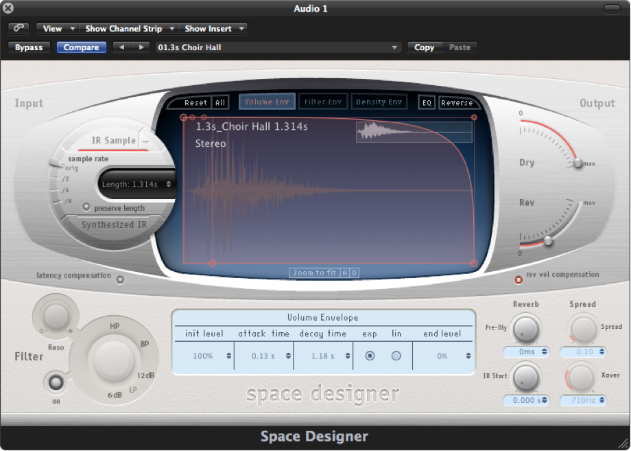
The reverb processor pictured in Figure 7.8 is based on a complex computation of delays and filters that achieve the effects requested by its control settings. Reverbs such as these are often referred to as algorithmic reverbs, after their unique mathematical designs.

[aside]Convolution is a mathematical process that operates in the time-domain – which means that the input to the operation consists of the amplitudes of the audio signal as they change over time. Convolution in the time-domain has the same effect as mathematical filtering in the frequency domain, where the input consists of the magnitudes of frequency components over the frequency range of human hearing. Filtering can be done in either the time domain or the frequency domain, as will be explained in Section 3.[/aside]

There is another type of reverb processor called a convolution reverb, which creates its effect using an entirely different process. A convolution reverb processor uses an impulse response (IR) captured from a real acoustic space, such as the one shown in Figure 7.8. An impulse response is essentially the recorded capture of a sudden burst of sound as it occurs in a particular acoustical space. If you were to listen to the IR, which in its raw form is simply an audio file, it would sound like a short “pop” with somewhat of a unique timbre and decay tail. The impulse response is applied to an audio signal by a process known as convolution, which is where this reverb effect gets its name. Applying convolution reverb as a filter is like passing the audio signal through a representation of the original room itself. This makes the audio sound as if it were propagating in the same acoustical space as the one in which the impulse response was originally captured, adding its reverberant characteristics.

With convolution reverb processors, you lose the extra control provided by the traditional pre-delay, early reflections, and RT60 parameters, but you often gain a much more natural reverberant effect. Convolution reverb processors are generally more CPU intensive than their more traditional counterparts, but with the speed of modern CPUs, this is not a big concern. Figure 7.8 shows an example of a convolution reverb plug-in.

7.1.10.1 Amplitude Adjustment and Normalization

One of the most straightforward types of audio processing is amplitude adjustment – something as simple as turning up or down a volume control. In the analog world, a change of volume is achieved by changing the voltage of the audio signal. In the digital world, it’s achieved by adding to or subtracting from the sample values in the audio stream – just simple arithmetic.

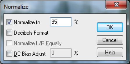
An important form of amplitude processing is normalization, which entails increasing the amplitude of the entire signal by a uniform proportion. Normalizers achieve this by allowing you to specify the maximum level you want for the signal, in percentages or dB, and increasing all of the samples’ amplitudes by an identical proportion such that the loudest existing sample is adjusted up or down to the desired level. This is helpful in maximizing the use of available bits in your audio signal, as well as matching amplitude levels across different sounds. Keep in mind that this will increase the level of everything in your audio signal, including the noise floor.

7.1.10.2 Dynamics Compression and Expansion

[wpfilebase tag=file id=141 tpl=supplement /]

Dynamics processing refers to any kind of processing that alters the dynamic range of an audio signal, whether by compressing or expanding it. As explained in Chapter 5, the dynamic range is a measurement of the perceived difference between the loudest and quietest parts of an audio signal. In the case of an audio signal digitized in n bits per sample, the maximum possible dynamic range is computed as the logarithm of the ratio between the loudest and the quietest measurable samples – that is, $$20\log_{10}\left ( \frac{2^{n-1}}{1/2} \right )dB$$. We saw in Chapter 5 that we can estimate the dynamic range as 6n dB. For example, the maximum possible dynamic range of a 16-bit audio signal is about 96 dB, while that of an 8-bit audio signal is about 48 dB.

The value of $$20\log_{10}\left ( \frac{2^{n-1}}{1/2} \right )dB$$ gives you an upper limit on the dynamic range of a digital audio signal, but a particular signal may not occupy that full range. You might have a signal that doesn’t have much difference between the loudest and quietest parts, like a conversation between two people speaking at about the same level. On the other hand, you might have at a recording of a Rachmaninoff symphony with a very wide dynamic range. Or you might be preparing a background sound ambience for a live production. In the final analysis, you may find that you want to alter the dynamic range to better fit the purposes of the recording or live performance. For example, if you want the sound to be less obtrusive, you may want to compress the dynamic range so that there isn’t such a jarring effect from a sudden difference between a quiet and a loud part.

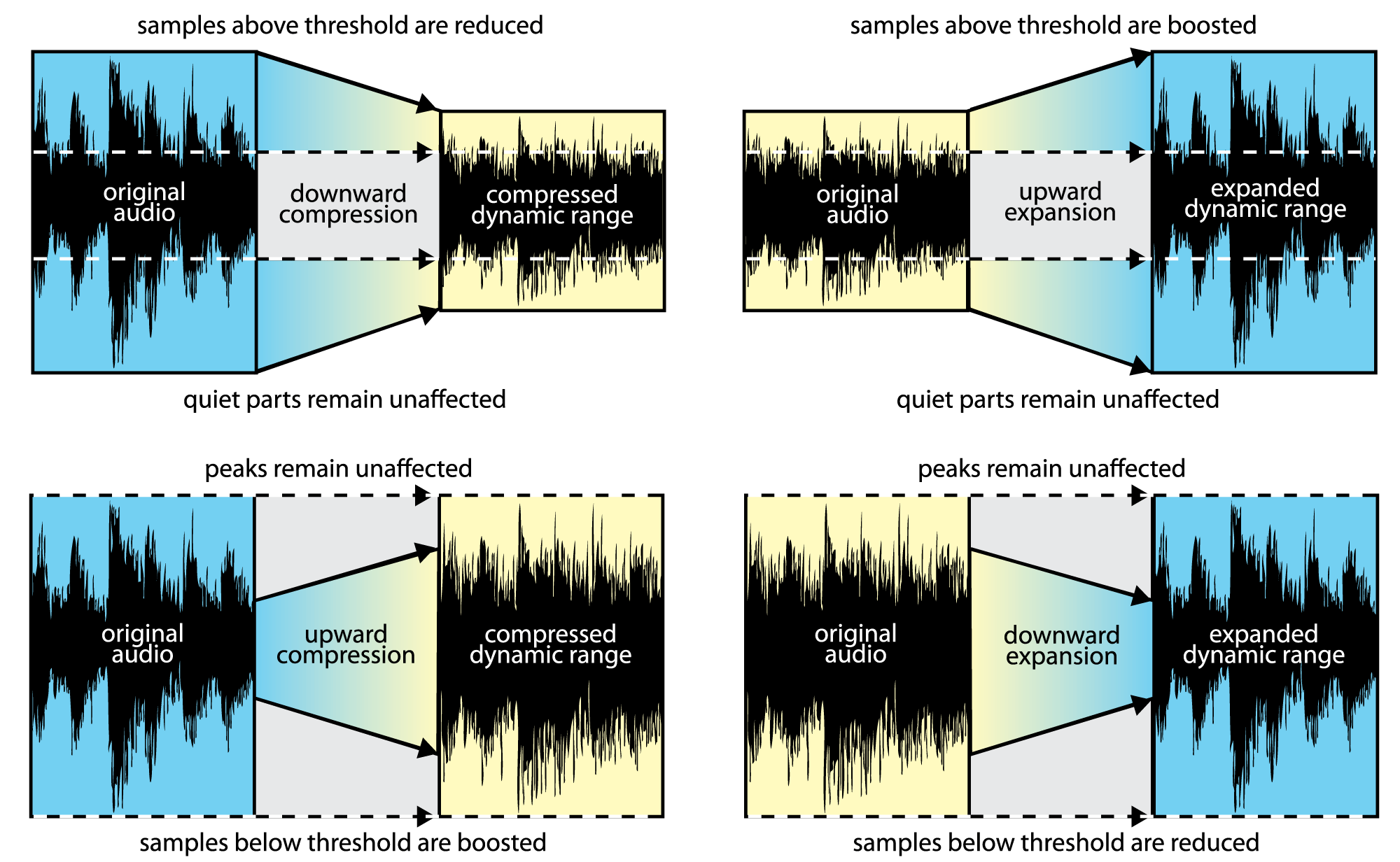
In dynamics processing, the two general possibilities are compression and expansion, each of which can be done in the upwards or downwards direction (Figure 7.13). Generally, compression attenuates the higher amplitudes and boosts the lower ones, the result of which is less difference in level between the loud and quiet parts, reducing the dynamic range. Expansion generally boosts the high amplitudes and attenuates the lower ones, resulting in an increase in dynamic range. To be precise:

• Downward compression attenuates signals that are above a given threshold, not changing signals below the threshold. This reduces the dynamic range.
• Upward compression boosts signals that are below a given threshold, not changing signals above the threshold. This reduces the dynamic range.
• Downward expansion attenuates signals that are below a given threshold, not changing signals above the threshold. This increases the dynamic range.
• Upward expansion boosts signals that are above a given threshold, not changing signals below the threshold. This increases the dynamic range.

The common parameters that can be set in dynamics processing are the threshold, attack time, and release time. The threshold is an amplitude limit on the input signal that triggers compression or expansion. (The same threshold triggers the deactivation of compression or expansion when it is passed in the other direction.) The attack time is the amount of time allotted for the total amplitude increase or reduction to be achieved after compression or expansion is triggered. The release time is the amount of time allotted for the dynamics processing to be “turned off,” reaching a level where a boost or attenuation is no longer being applied to the input signal.

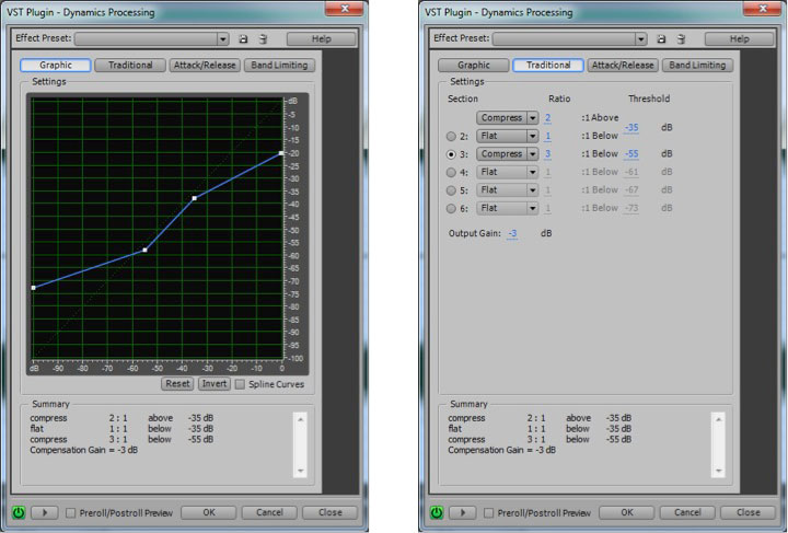
Adobe Audition has a dynamics processor with a large amount of control. Most dynamics processor’s controls are simpler than this – allowing only compression, for example, with the threshold setting applying only to downward compression. Audition’s processor allows settings for compression and expansion and has a graphical view, and thus it’s a good one to illustrate all of the dynamics possibilities.

Figure 7.14 shows two views of Audition’s dynamics processor, the graphic and the traditional, with settings for downward and upward compression. The two views give the same information but in a different form.

In the graphic view, the unprocessed input signal is on the horizontal axis, and the processed input signal is on the vertical axis. The traditional view shows that anything above -35 dBFS should be compressed at a 2:1 ratio. This means that the level of the signal above -35 dBFS should be reduced by ½ . Notice that in the graphical view, the slope of the portion of the line above an input value of -35 dBFS is ½. This slope gives the same information as the 2:1 setting in the traditional view. On the other hand, the 3:1 ratio associated with the -55 dBFS threshold indicates that for any input signal below -55 dBFS, the difference between the signal and -55 dBFS should be reduced to 1/3 the original amount. When either threshold is passed (-35 or -55 dBFS), the attack time (given on a separate panel not shown) determines how long the compressor takes to achieve its target attenuation or boost. When the input signal moves back between the values of -35 dBFS and -55 dBFS, the release time determines how long it takes for the processor to stop applying the compression.

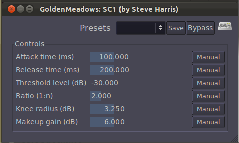
A simpler compressor – one of the ARDOUR LADSPA plug-ins, is shown in Figure 7.15. In addition to attack, release, threshold, and ratio controls, this compressor has knee radius and makeup gain settings. The knee radius allows you to shape the attack of the compression to something other than linear, giving a potentially smoother transition when it kicks in. The makeup gain setting (often called simply gain) allows you to boost the entire output signal after all other processing has been applied.

7.1.10.3 Limiting and Gating

[aside]A limiter could be thought of as a compressor with a compression ratio of infinity to 1.  See the next section on dynamics compression.[/aside]

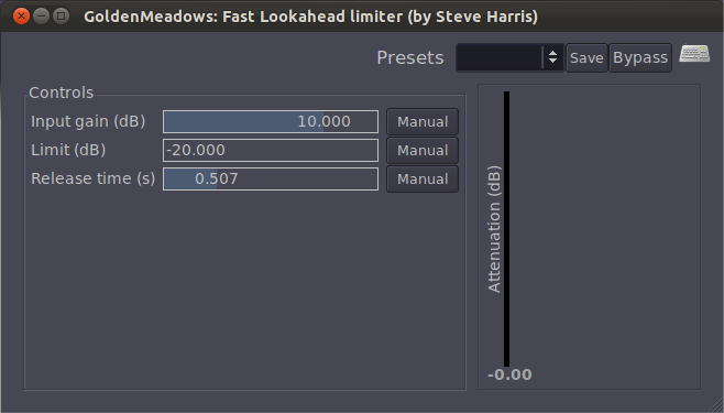
A limiter is a tool that prevents the amplitude of a signal from going over a given level. Limiters are often applied on the master bus, usually post-fader. Figure 7.16 shows the LADSPA Fast Lookahead Limiter plug-in. The input gain control allows you to increase the input signal before it is checked by the limiter. This limiter looks ahead in the input signal to determine if it is about to go above the limit, in which case the signal is attenuated by the amount necessary to bring it back within the limit. The lookahead allows the attenuation to happen almost instantly, and thus there is no attack time. The release time indicates how long it takes to go back to 0 attenuation when limiting the current signal amplitude is no longer necessary. You can watch this work in real-time by looking at the attenuation slider on the right, which bounces up and down as the limiting is put into effect.

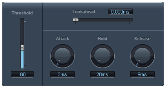
A gate allows an input signal to pass through only if it is above a certain threshold. A hard gate has only a threshold setting, typically a level in dB above or below which the effect is engaged. Other gates allow you to set an attack, hold, and release time to affect the opening, holding, and closing of the gate (Figure 7.18). Gates are sometimes used for drums or other instruments to make their attacks appear sharper and reduce the bleed from other instruments unintentionally captured in that audio signal.

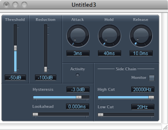
A noise gate is a specially designed gate that is intended to reduce the extraneous noise in a signal. If the noise floor is estimated to be, say, -80 dBFS, then a threshold can be set such that anything quieter than this level is blocked out, effectively transmitted as silence. A hysteresis control on a noise gate indicates that there is a threshold difference between opening and closing the gate. In the noise gate in Figure 7.18, the threshold of -50 dB and the hysteresis setting of -3 dB indicate that the gate closes at -50 dBFS and opens again at -47 dBFS. The side chain controls allow some signal other than the main input signal to determine when the input signal is gated. The side chain signal could cause the gate to close based on the amplitudes of only the high frequencies (high cut) or low frequencies (low cut).

In a practical sense, there is no real difference between a gate and a noise gate. A common misconception is that noise gates can be used to remove noise in a recording. In reality all they can really do is mute or reduce the level of the noise when only the noise is present. Once any part of the signal exceeds the gate threshold, the entire signal is allowed through the gate, including the noise. Still, it can be very effective at clearing up the audio in between words or phrases on a vocal track, or reducing the overall noise floor when you have multiple tracks with active regions but no real signal, perhaps during an instrumental solo.

[wpfilebase tag=file id=135 tpl=supplement /]

An equalizer can be incredibly useful when used appropriately, and incredibly dangerous when used inappropriately. Knowing when to use an EQ is just as important and knowing how to use it to accomplish the effect you are looking for. Every time you think you want to use an EQ you should evaluate the situation against this rule of thumb: EQ should be used to create an effect, not to solve a problem. Using an EQ as a problem solver can cause new problems when you should really just figure out what’s causing the original problem and fix that instead. Only if the problem can’t be solved in any other way should you pull up the EQ – for example, if you’re working post-production on a recording captured earlier during a film shoot, or you’ve run into an acoustical issue in a space that can’t be treated or physically modified. Rather than solving problems, you should try to use an EQ as a tool to achieve a certain kind of sound. Do you like your music to be heavy on the bass? An EQ can help you achieve this. Do you really like to hear the shimmer of the cymbals in a drum set? An EQ can help.

Let’s examine some common problems you may encounter where you might be tempted to use an EQ inappropriately. As you listen to the recording you’re making of a singer you notice that the recorded audio has a lot more low frequency than high frequency content, leading to a decreased intelligibility. You go over and stand next to the performer to hear what he actually sounds like and notice that he sounds quite different than what you’re hearing from the microphone. Standing next to him, you can hear all those high frequencies quite well. In this situation you may be tempted to pull out your EQ and insert a high shelf filter to boost all those high frequencies. This should be your last resort. Instead, you might notice that the singer is singing into the side of the microphone instead of the front. Because microphones are more directional at high frequencies than low frequencies, singing into the side of the microphone would mean that the microphone picks up the low frequency content very easily but the high frequencies are not being captured very well. In this case you would be using an EQ to boost something that isn’t being picked up very well in the first place. You will get much better results by simply rotating the microphone so it is pointed directly at the singer so the singer is singing into the part of the microphone that is more sensitive to high frequencies.

Another situation you may encounter would be when mixing the sound from multiple microphones either for a live performance or a recording. You notice as you start mixing everything together that a certain instrument has a huge dip around 250 Hz. You might be tempted to use an EQ to increase 250 Hz. The important thing to keep in mind here is that most microphones are able to pick up 250 Hz quite well from every direction, and it is unlikely that the instrument itself is somehow not generating the frequencies in the 250 Hz range while still generating all the other frequencies reasonably well. So before you turn on that EQ, you should mute all the other channels on the mixer and listen to the instrument alone. If the problem goes away, you know that whatever is causing the problem has nothing to do with EQ. In this situation, comb filtering is the likely culprit. There’s another microphone in your mix that was nearby and happened to be picking up this same instrument at a slightly longer distance of about two feet. When you mix these two microphones together, 250 Hz is one of the frequencies that cancels out. If comb filtering is the issue, you should try to better isolate the signals either by moving the microphones farther apart or preventing them from being summed together in the mix. A gate might come in handy here, too. If you gate both signals you can minimize the times when both microphones are mixed together, since the signals won’t be let through when the instruments they are being used for aren’t actually playing.

If comb filtering isn’t the issue, try moving a foot or two closer to or farther away from the loudspeakers. If the 250 Hz dip goes away in this case, there’s likely a standing wave resonance in your studio at the mix position that is cancelling out this frequency. Using an EQ in this case will not solve the problem since you’re trying to boost something that is actively being cancelled out. A better solution for the standing wave would be to consider rearranging your room or applying acoustical treatment to the offending surfaces that are causing this reflective build up.

Suppose you are operating a sound reinforcement system for a live performance and you start getting feedback through the sound system. When you hear that single frequency start its endless loop through the system you might be tempted to use an EQ to pull that frequency out of the mix. This will certainly stop the feedback, but all you really get is the ability to turn the system up another decibel or so before another frequency will inevitably start to feed back. Repeat the process a few times and in no time at all you will have completely obliterated the frequency response of your sound system. You won’t have feedback, but the entire system will sound horrible. A better strategy for solving this problem would be to get the microphone closer to the performer, and move the performer and the microphone farther away from the loudspeakers. You’ll get more gain this way and you can maintain the frequency response of your system. (Chapter 4 has moree on potential acoustic gain. Chapter 8 has an exercise on gain setting.)

We could examine many more examples of an inappropriate use of an EQ but they all go back to the rule of thumb regarding the use of an EQ as a problem solver. In most cases, an EQ is a very ineffective problem solver. It is, however, a very effective tool for shaping the tonal quality of a sound. This is an artistic effect that has little to do with problems of a given sound recording or reinforcement system. Instead you are using the EQ to satisfy a certain tonal preference for the listener. These effects could be as subtle as reducing an octave band of frequencies around 500 Hz by -3 dB to achieve more intelligibility for the human voice by allowing the higher frequencies to be more prominent. The effect could be as dramatic as using a bandpass filter to mimic the effect of a small cheap loudspeaker in a speakerphone. When using an EQ as an effect, keep in mind another rule of thumb. When using an EQ, you should reduce the frequencies that are too loud instead of increasing the frequencies that are too quiet. Every sound system, whether in a recording studio or a live performance, has an amplitude ceiling – the point at which the system clips and distorts. If you’ve done your job right, you will be running the sound system at an optimal gain, and a 3 dB boost of a given frequency on an EQ could be enough to cause a clipped signal. Reducing frequencies is always safer than boosting them since reducing them will not blow the gain structure in your signal path.

[aside]In an attempt to reconcile these two schools of thought on reverberation in the recording studio, some have resorted to installing active acoustic systems in the recording studio. These systems involve placing microphones throughout the room that feed into live digital signal processors that generate thousands of delayed sounds that are then sent into several loudspeakers throughout the room. This creates a natural-sounding artificial reverb that is captured in the recording the same as natural reverb. The advantage here is that you can change the reverb by adjusting the parameters of the DSP for different recording situations. To hear an example of this kind of system in action, see this video from TRI Studios where Bob Weir from the Grateful Dead has installed an active acoustic system in his recording studio.[/aside]

Almost every audio project you do will likely benefit from some reverb processing. In a practical sense, most of the isolation strategies we use when recording sounds will have a side effect of stripping the sound of natural reverberation. So anything recorded in a controlled environment such as a recording studio will probably need some reverb added to make it sound more natural. There are varying opinions on this among audio professionals. Some argue that artificial reverberation processers are sounding quite good now, and since it is impossible to remove natural reverberation from a recording, it makes more sense to capture your recorded audio as dry as possible. This way you’re able to artificially add back whatever reverberation you need in a way that you can control. Others argue that having musicians perform in an acoustically dry and isolated environment will negatively impact the quality of their performance. Think about how much more confident you feel when singing in the shower. All that reverberation from the tiled surfaces in the shower create a natural reverberation that makes your voice sound better to you than normal. That gives you the confidence to sing in a way that you probably don’t in public. So some recording engineers would prefer to have some natural reverberation in the recording room to help the musicians to deliver a better performance. If that natural reverberation is well controlled acoustically you could even end up with a recording that sounds pretty good already and might require minimal additional processing.

Regardless of the amount of reverb you already have in your recording, you will likely still want to add some artificial reverb to the mix. There are three places you can apply the reverb in your signal chain. You can set it up as an insert for a specific channel in a multi-channel mix. In this case the reverb only gets applied to the one specific channel, and the other channels are left unchanged. You have to adjust the wet/dry mix in the reverb processor to create an appropriate balance. This technique can be useful for a special effect you want to put on a specific sound, but using this technique on every channel in a large multi-channel mix costs you a lot in CPU performance because the multiple reverb processors that are running simultaneously. If you have a different reverb setting on each channel you could also have a rather confusing mix since every sound will seem to be in a different acoustic environment. Maybe that’s what you want if you’re creating a dream sequence or something abstract for a play or film, but for a music recording it usually makes more sense to have every instrument sounding like it is in the same room.

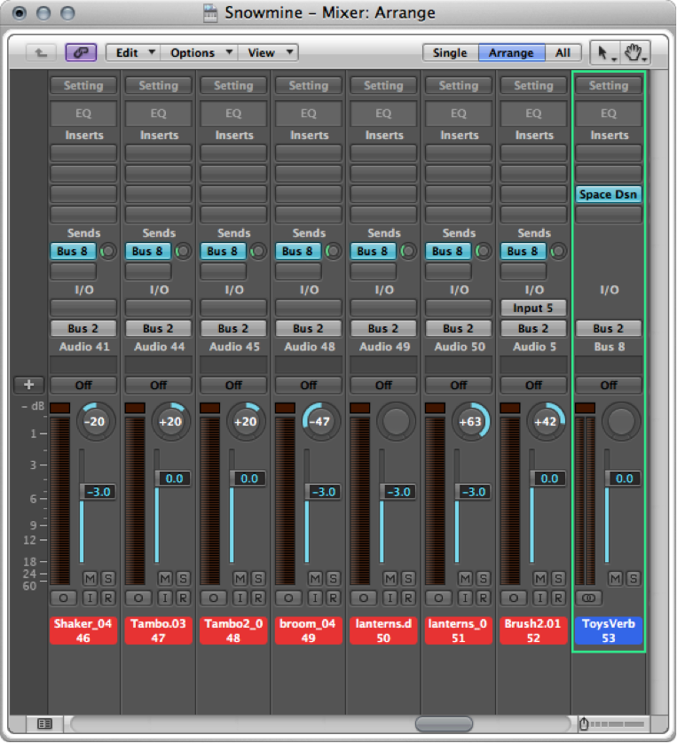
The second reverb technique can solve both the problem of CPU performance and varying acoustic signatures. In this case you would set up a mix bus that has a reverb inserted. You would set the reverb processor to 100% wet. This basically becomes the sound of your virtual room. Then you can set up each individual channel in your mix to have a variable aux send that dials in a certain amount of the signal into the reverb bus. In other words, the individual sends decide how much that instrument interacts with your virtual room. The individual channel will deliver the dry sound to the mix and the reverb bus will deliver the wet. The amount of sound that is sent on the variable aux send determines the balance of wet to dry. This strategy allows you to send many different signals into the reverb processor at different levels and therefore have a separate wet/dry balance for each signal, while using only one reverberation processor. The overall wet mix can also be easily adjusted using the fader on the aux reverb bus channel. This technique is illustrated in Figure 7.30.

The third strategy for applying reverberation is to simply apply a single reverb process to an entire mix output. This technique is usually not preferred because you have no control over the reverb balance between the different sounds in the mix. The reason you would use this technique is if you don’t have access to the raw tracks or if you are trying to apply a special reverb effect to a single audio file. In this case just pick a reverb setting and adjust the wet/dry mix until you achieve the sound you are looking for.

The most difficult task in using reverb is to find the right balance. It is very easy to overdo the effect. The sound of reverberation is so intoxicating that you have to constantly fight the urge to apply the effect more dramatically. Before you commit to any reverb effect, listen to it though a few different speakers or headphones and in a few different listening environments. A reverb effect sounds like a good balance in one environment might sound over the top in another. Listen to other mixes of similar music or sound to compare your work with the work of seasoned professionals. Before long you’ll develop a sixth sense for the kind of reverb to apply in a given situation.

When deciding whether to use dynamics processing you should keep in mind that a dynamics processor is simply an automatic volume knob. Any time you find yourself constantly adjusting the level of a sound, you may want to consider using some sort of dynamics processor to handle that for you. Most dynamics processors are in the form of downwards compressors. These compressors work by reducing the level of sounds that are too loud but letting quieter sounds pass without any change in level.

[aside]There is some disagreement among audio professionals about the use of compressors. There are some who consider using a compressor as a form of cheating. Their argument is that no compressor can match the level of artistry that can be accomplished by a skilled mixer with their fingers on the faders. In fact, if you ask some audio mix engineers which compressors they use, they will respond by saying that they have ten compressors and will show them to you by holding up both hands and wiggling their fingers![/aside]

One example when compression can be helpful is when mixing multiple sounds together from a multitrack recording. The human voice singing with other instruments is usually a much more dynamic sound than the other instruments. Guitars and basses, for example are not known as particularly dynamic instruments. A singer is constantly changing volume throughout a song. This is one of the tools a singer uses to produce an interesting performance. When mixing a singer along with the instruments from a band, the band essentially creates a fairly stable noise floor. The word noise is not used here in a negative context; rather, it is used to describe a sound that is different from the vocal that has the potential of masking the vocal if there is not enough difference in level between the two. As a rule of thumb, for adequate intelligibility of the human voice, the peaks of the voice signal need to be approximately 25 dB louder than the noise floor, which in this case is the band. It is quite possible for a singer to perform with a 30 dB dynamic range. In other words, the quietest parts of the vocal performance are 30 dB quieter than the loudest parts of the vocal performance.

If the level of the band is more or less static and the voice is moving all around, how are you going to maintain that 25 dB ratio between the peaks of the voice and the level of the band? In this situation you will never find a single level for the vocal fader that will allow it to be heard and understood consistently throughout the song. You could painstakingly draw in a volume automation curve in your DAW software, or you could use a compressor to do it for you. If you can set the threshold somewhere in the middle of the dynamic range of the vocal signal and use a 2:1 or 4:1 compression ratio, can easily turn that 30 dB of dynamic range into a 20 dB range or less. Since the compressor is turning down all the loud parts, the compressed signal will sound much quieter than the uncompressed signal, but if you turn the signal up using either the output gain of the compressor or the channel fader you can bring it back to a better level. With the compressed signal, you can now much more easily find a level for the voice that allows it to sit well in the mix. Depending on how aggressive you are about the compression, you may still need to automate a few volume changes, but the compressor has helped turn a very difficult to solve problem into something more manageable.

Rather than using a compressor to allow a sound to more easily take focus over a background sound, you can also use compression as a tool for getting a sound to sit in the mix in a way that allows other sounds to take focus. This technique is used often in theatre and film for background music and sound effects. The common scenario is when a sound designer or composer tries to put in some underscore music or background sounds into a scene for a play or a film and the director inevitably says, “turn it down, it’s too loud.” You turn it down by 6 dB or so and the director still thinks it’s too loud. By the time you turn it down enough to satisfy the director, you can hardly hear the sound and before long, you’ll be told to simply cut it because it isn’t contributing to the scene in any meaningful way.

The secret to solving this problem is often compression. When the director says the sound is too loud, what he really means is that the sound is too interesting. More interesting than the actor, in fact, and consequently the audience is more likely to pay attention to the music or the background sound than they are to the actor. One common culprit when a sound is distracting is that it is too dynamic. If the music is constantly jumping up and down in level, it will draw your focus. Using a compressor to make the underscore music or background sounds less dynamic allows them to sit in the mix and enhance the scene without distracting from the performance of the actor.

Compression can be a useful tool, but like any good thing, if it’s overused compression can be detrimental to the quality of your sound. Dynamics are one quality of sound and music that makes it exciting, interesting, and evocative. A song with dynamics that have been completely squashed will not be very interesting to listen to and can cause great fatigue on the ears. Also, if you apply compression inappropriately, it may cause audible artifacts in the sound, where you can hear when the sound is being attenuated and released. This is referred to as “pumping” or “breathing,” and it usually means you’ve taken the compression too far or in the wrong direction. So you have to be very strategic about the use of compression and go easy on the compression ratio. Often, a mild compression ratio is enough to tame an overly dynamic sound without completely stripping it of all its character.