6.1.3 MIDI Data Compared to Digital Audio
Consider how MIDI data differs from digital audio as described in Chapter 5. You aren’t recording something through a microphone. MIDI keyboards don’t necessarily make a sound when you strike a key on a piano keyboard-like controller, and they don’t function as stand-alone instruments. There’s no sampling and quantization going on at all. Instead, the controller is engineered to know that when a certain key is played, a symbolic message should be sent detailing the performance information.
[aside]Many systems interpret a Note On message with velocity 0 as “note off” and use this as an alternative to the Note Off message.[/aside]
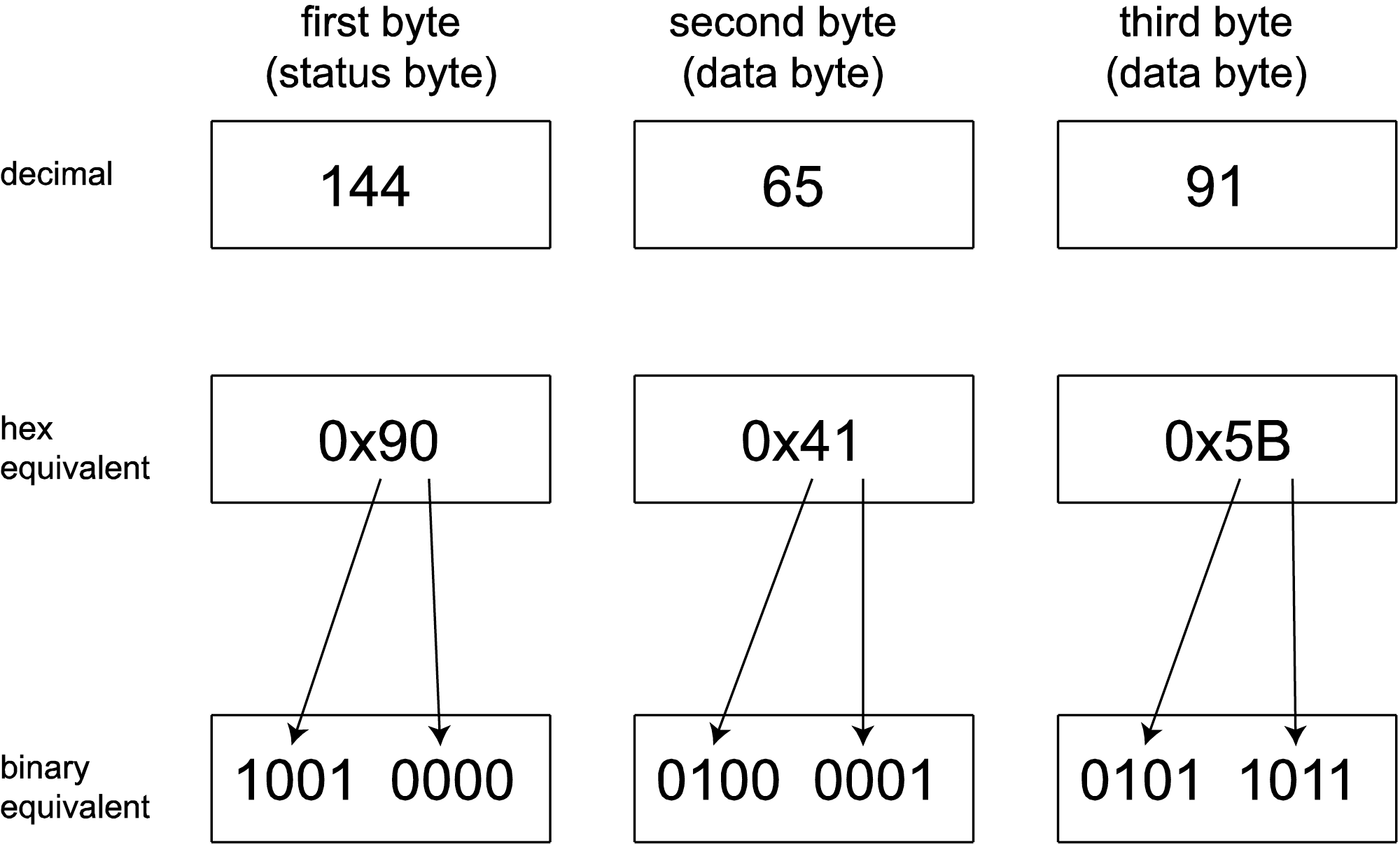
In the case of a key press, the MIDI message would convey the occurrence of a Note On, followed by the note pitch played (e.g., middle C) and the velocity with which it was struck. The MIDI message generated by this action is only three bytes long. It’s essentially just three numbers, as shown in Figure 6.7. The first byte is a value between 144 and 159. The second and third bytes are values between 0 and 127. The fact that the first value is between 144 and 159 is what makes it identifiable by the receiver as a Note On message, and the fact that it is a Note On message is what identifies the next two bytes as the specific note and velocity. A Note Off message is handled similarly, with the first byte identifying the message as Note Off and the second and third giving note and velocity information (which can be used to control note decay).
Let’s say that the key is pressed and a second later it is released. Thus, the playing of a note for one second requires six bytes. (We can set aside the issue of how the time between the notes is stored symbolically, since it’s handled at a lower level of abstraction.) How does this compare to the number of bytes required for digital audio? One second of 16-bit mono audio at a sampling rate of 44,100 Hz requires 44,100 samples/s * 2 bytes/sample = 88,200 bytes/s. Clearly, MIDI can provide a more concise encoding of sound than digital audio.
MIDI differs from digital audio in other significant ways as well. A digital audio recording of sound tries to capture the sound exactly as it occurs by sampling the sound pressure amplitude over time. A MIDI file, on the other hand, records only symbolic messages. These messages make no sound unless they are interpreted to do so by a synthesizer. When we speak of a MIDI “recording,” we mean it only in the sense that MIDI data has been captured and stored – not in the sense that sound has actually been recorded. While MIDI messages are most frequently interpreted and synthesized into musical sounds, they can be interpreted in other ways (as we’ll illustrate in Section 6.1.8.5.3). The messages mean only what the receiver interprets them to mean.
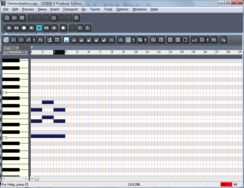
With this caveat in mind, we’ll continue from here under the assumption that you’re using MIDI primarily for music production since this is MIDI’s most common application. When you “record” MIDI music via a keyboard controller, you’re saving information about what notes to play, how hard or fast to play them, how to modulate them with pitch bend or with a sustain pedal, and what instrument the notes should sound like upon playback. If you already know how to read music and play the piano, you can enjoy the direct relationship between your input device – which is essentially a piano keyboard – and the way it saves your performance – the notes, the timing, even the way you strike the keys if you have a velocity-sensitive controller. Many MIDI sequencers have multiple ways of viewing your file, including a track view, a piano roll view, an event list view, and even a staff view – which shows the notes that you played in standard music notation. These are shown in Figure 6.8 through Figure 6.11.


[aside]The word sample has different meanings in digital audio and MIDI. In MIDI, a sample is a small sound file representing a single instance of sound made by some instrument, like a note played on a flute.[/aside]
MIDI and digital audio are simply two different ways of recording and editing sound – with an actual real-time recording or with a symbolic notation. They serve different purposes. You can actually work with both digital audio and MIDI in the same context, if both are supported by the software. Let’s look more closely now at how this all happens.Another significant difference between digital audio and MIDI is the way in which you edit them. You can edit uncompressed digital audio down to the sample level, changing the values of individual samples if you like. You can requantize or resample the values, or process them with mathematical operations. But always they are values representing changing air pressure amplitude over time. With MIDI, you have no access to individual samples, because that’s not what MIDI files contain. Instead, MIDI files contain symbolic representations of notes, key signatures, durations of notes, tempo, instruments, and so forth, making it possible for you to edit these features with a simple menu selection or an editing tool. For example, if you play a piece of music and hit a few extra notes, you can get rid of them later with an eraser tool. If your timing is a little off, you can move notes over or shorten them with the selection tool in the piano roll view. If you change your mind about the instrument sound you want or the key you’d like the piece played in, you can change these with a click of the mouse. Because the sound has not actually been synthesized yet, it’s possible to edit its properties at this high level of abstraction.
6.1.4 Channels, Tracks, and Patches in MIDI Sequencers
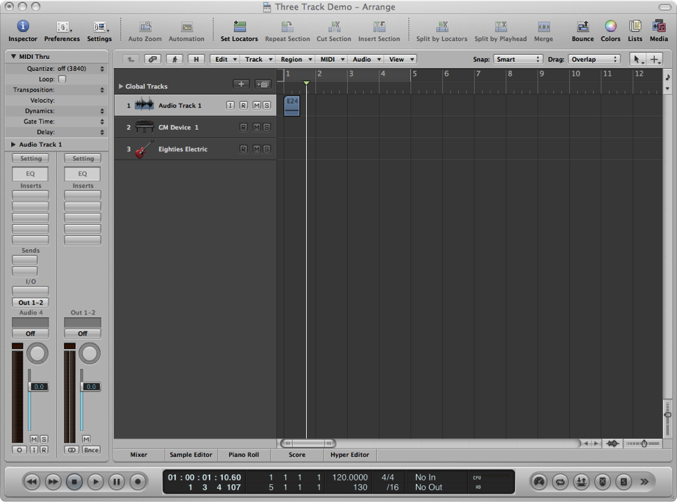
A software MIDI sequencer serves as an interface between the input and output. A track is an editable area on your sequencer interface. You can have dozens or even hundreds of tracks in your sequencer. Tracks are associated with areas in memory where data is stored. In a multitrack editor, you can edit multiple tracks separately, indicating input, output, amplitude, special effects, and so forth separately for each. Some sequencers accommodate three types of tracks: audio, MIDI, and instrument. An audio track is a place to record and edit digital audio. A MIDI track stores MIDI data and is output to a synthesizer, either a software device or to an external hardware synth through the MIDI output ports. An instrument track is essentially a MIDI track combined with an internal soft synth, which in turn sends its output to the sound card. It may seem like there isn’t much difference between a MIDI track and an instrument track. The main difference is that the MIDI track has to be more explicitly linked to a hardware or software synthesizer that produces its sound, whereas an instrument track has the synth, in a sense, “embedded” in it. Figure 6.12 shows each of these types of tracks.
A channel is a communication path. According to the MIDI standard, a single MIDI cable can transmit up to 16 channels. Without knowing the details of how this is engineered, you can just think of it abstractly as 16 separate lines of communication.
There are both input and output channels. An incoming message can tell what channel it is to be transmitted on, and this can route the message to a particular device. In the sequencer pictured in Figure 6.13, track 1 is listening on all channels, indicated by the word OMNI. Track 2 is listening only on Channel 2.
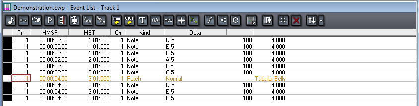
The output channels are pointed out in the figure, also. When the message is sent out to the synthesizer, different channels can correspond to different instrument sounds. The parameter setting marked with a patch cord icon is the patch. A patch is a message to the synthesizer – just a number that indicates how the synthesizer is to operate as it creates sounds. The synthesizer can be programmed in different ways to respond to the patch setting. Sometimes the patch refers to a setting you’ve stored in the synthesizer that tells it what kinds of waveforms to combine or what kind of special effects to apply. In the example shown in Figure 6.13, however, the patch is simply interpreted as the choice of instrument that the user has chosen for the track. Track 1 is outputting on Channel 1 with the patch set to Acoustic Grand Piano. Track 2 is outputting on Channel 2 with the patch set to Cello.
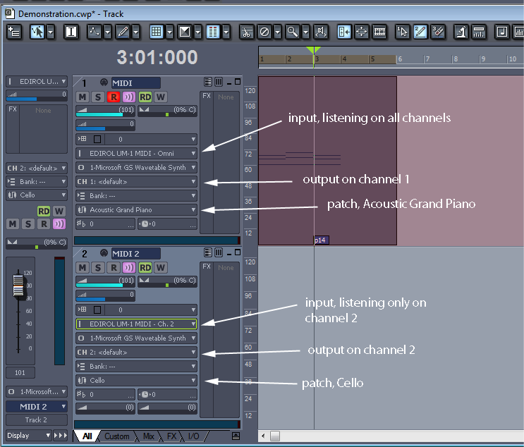
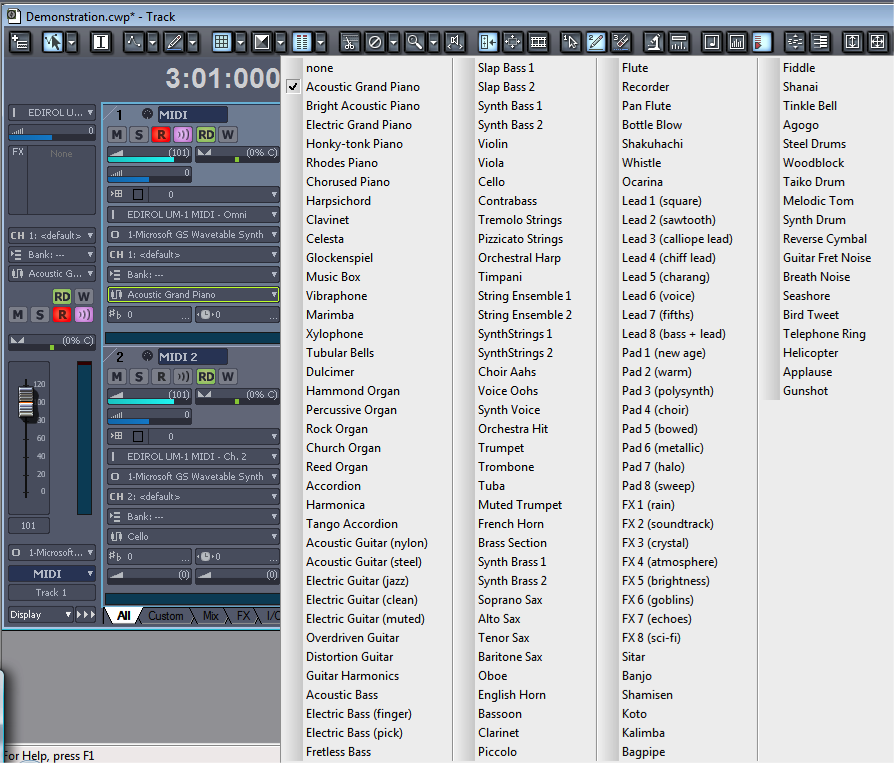
It’s possible to call for a patch change by means of the Program Change MIDI message. This message sends a number to the synthesizer corresponding to the index of the patch to load. A Program Change message is inserted into track 1 in Figure 6.13. You can see a little box with p14 in it at the bottom of the track indicating that the synth should be changed to patch 14 at that point in time. This is interpreted as changing the instrument patch from a piano to tubular bells. In the setup pictured, we’re just using the Microsoft GS Wavetable Synth as opposed to a more refined synth. For the computer’s built-in synth, the patch number is interpreted according to the General MIDI standard. The choices of patches in this standard can be seen when you click on the drop down arrow on the patch parameter, as shown in Figure 6.14. You can see that the fifteenth patch down the list is tubular bells. (The Program Change message is still 14 because the numbering starts at 0.)
In a later section in this chapter, we’ll look at other ways that the Program Change message can be interpreted by a synthesizer.
6.1.5 A Closer Look at MIDI Messages
6.1.5.1 Binary, Decimal, and Hexadecimal Numbers
When you read about MIDI message formats or see them in software interfaces, you’ll find that they are sometimes represented as binary numbers, sometimes as decimal numbers, and sometimes as hexadecimal numbers (hex, for short), so you should get comfortable moving from one base to another. Binary is base 2, decimal is base 10, and hex is base 16. You can indicate the base of a number with a subscript, as in 011111002, 7C16, and 12410. Often, 0x is placed in front of hex numbers, as in 0x7C. Some sources use an H after a hex number, as in 7CH. Usually, you can tell by context what base is intended, and we’ll omit the subscript unless the context is not clear. We assume that you understand number bases and can convert from one to another. If not, you should easily be able to find a resource on this for a quick crash course.
Binary and hexadecimal are useful ways to represent MIDI messages because they allow us to divide the messages in meaningful groups. A byte is eight bits. Half a byte is four bits, called a nibble. The two nibbles of a MIDI message can encode two separate pieces of information. This fact becomes important in interpreting MIDI messages, as we’ll show in the next section. In both the binary and hexadecimal representations, we can see the two nibbles as two separate pieces of information, which isn’t possible in decimal notation.
A convenient way to move from hexadecimal to binary is to translate each nibble into four bits and concatenate them into a byte. For example, in the case of 0x7C, the 7 in hexadecimal becomes 0111 in binary. The C in hexadecimal becomes 1100 in binary. Thus 0x7C is 01111100 in binary. (Note that the symbols A through F correspond to decimal values 10 through 15, respectively, in hexadecimal notation.)
6.1.5.2 MIDI Messages, Types, and Formats
In Section 6.1.3, we showed you an example of a commonly used MIDI message, Note On, but now let’s look at the general protocol.
MIDI messages consist of one or more bytes. The first byte of each message is a status byte, identifying the type of message being sent. This is followed by 0 or more data bytes, depending on the type of message. Data bytes give more information related to the type of message, like note pitch and velocity related to Note On.
All status bytes have a 1 as their most significant bit, and all data bytes have a 0. A byte with a 1 in its most significant bit has a value of at least 128. That is, 10000000 in binary is equal to 128 in decimal, and the maximum value that an 8 bit binary number can have (11111111) is the decimal value 255. Thus, status bytes always have a decimal value between 128 and 255. This is 10000000 through 11111111 in binary and 80 through FF in hex.
[wpfilebase tag=file id=41 tpl=supplement /]
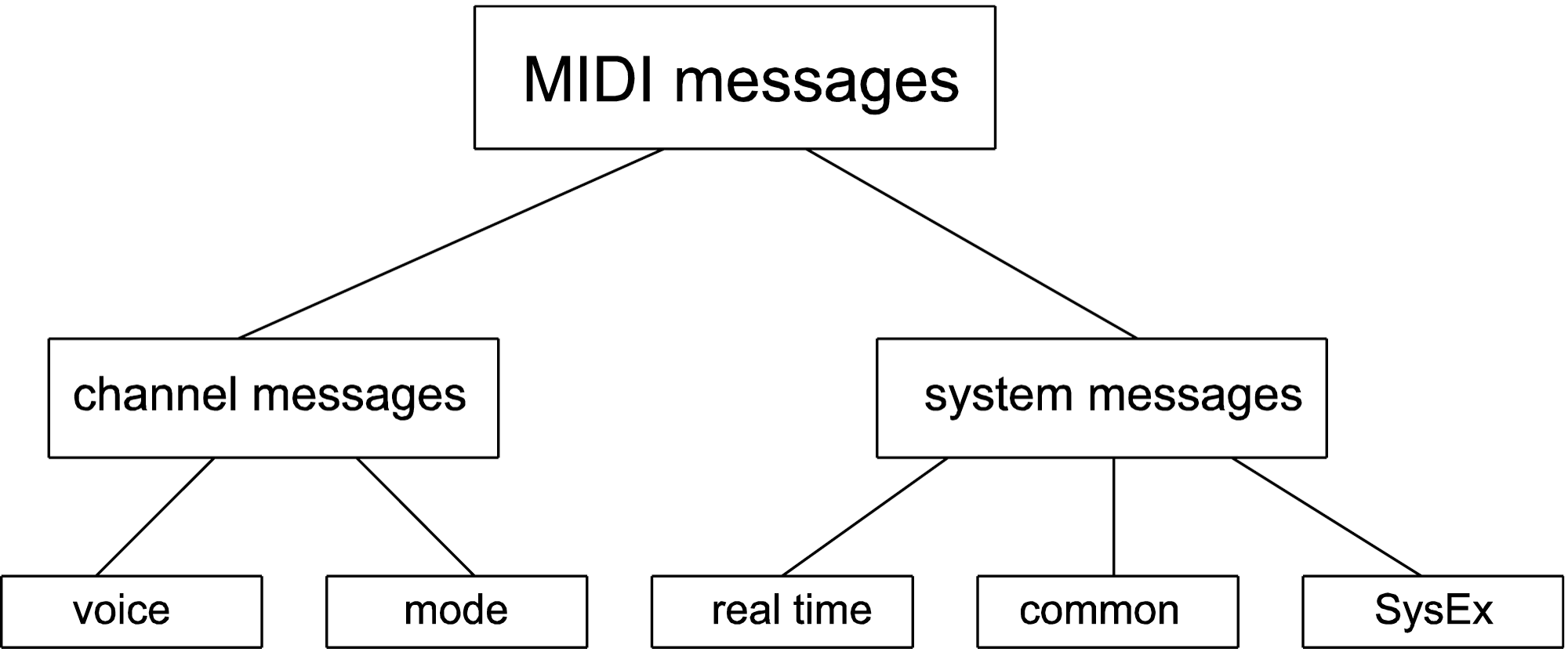
MIDI messages can be divided into two main categories: Channel messages and System messages. Channel messages contain the channel number. They can be further subdivided into voice and mode messages. Voice messages include Note On, Note Off, Polyphonic Key Pressure, Control Change, Program Change, Channel Pressure/Aftertouch, and Pitch Bend. A mode indicates how a device is to respond to messages on a certain channel. A device might be set to respond to all MIDI channels (called Omni mode), or it might be instructed to respond to polyphonic messages or only monophonic ones. Polyphony involves playing more than one note at the same time.
System messages are sent to the whole system rather than a particular channel. They can be subdivided into Real Time, Common, and System Exclusive messages (SysEx). The System Common messages include Tune Request, Song Select, and Song Position Pointer. The system real time messages include Timing Clock, Start, Stop, Continue, Active Sensing, and System Reset. SysEx messages can be defined by manufacturers in their own way to communicate things that are not part of the MIDI standard. The types of messages are diagrammed in Figure 6.15. A few of these messages are shown in Table 6.1.
[table caption=”Table 6.1 Examples of MIDI messages” width=”80%”]
Hexadecimal*,Binary**,Number of Data Bytes,Description
Channel Voice Messages[attr colspan=”4″ style=”text-align:center;font-weight:bold”]
8n,1000mmmm,2,Note Off
9n,1001mmmm,2,Note On
An,1010mmmm,2,Polyphonic Key Pressure/Aftertouch
Bn,1011mmmm,2,Control Change***
Cn,1100mmmm,1,Program Change
Dn,1101mmmm,1,Channel Pressure/Aftertouch
En,1110mmmm,2,Pitch Bend Change
Channel Mode Messages[attr colspan=”4″ style=”text-align:center;font-weight:bold”]
Bn,1101mmmm,2,Selects Channel Mode
System Messages[attr colspan=”4″ style=”text-align:center;font-weight:bold”]
F3,11110011,1,Song Select
F8,11111000,0,Timing Clock
F0,11110000,variable,System Exclusive
*Each n is a hex digit between 0 and F. [attr colspan=”4″]
**Each m is a binary digit between 0 and 1.[attr colspan=”4″]
***Channel Mode messages are a special case of Control Change messages. The difference is in the first data byte. Data byte values 0x79 through 0x7F have been reserved in the Control Change message for information about mode changes.[attr colspan=”4″]
[/table]
[wpfilebase tag=file id=124 tpl=supplement /]
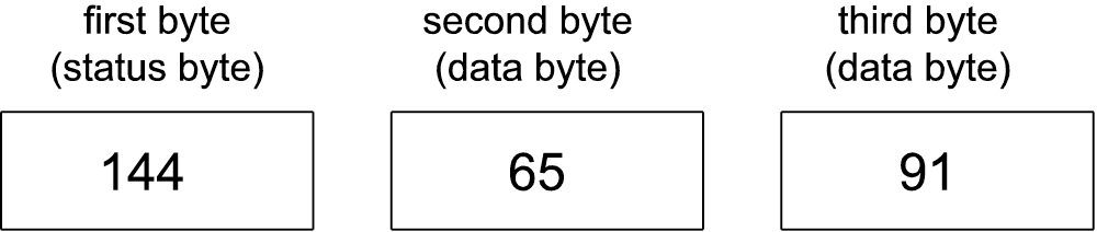
Consider the MIDI message shown in all three numerical bases in Figure 6.16. In the first byte, the most significant bit is 1, identifying this as a status byte. This a Note On message. Since it is a channel message, it has the channel in its least significant four bits. These four bits can range from 0000 to 1111, corresponding to channels 1 through 16. (Notice that the binary value is one less than the channel number as it appears on our sequencer interface. A Note On message with 0000 in the least significant nibble indicates channel 1, one with 0001 indicates channel 2, and so forth.)
A Note On message is always followed by two data bytes. Data bytes always have a most significant bit of 0. The note to be played is 0x41, which translates to 65 in decimal. By the MIDI standard, note 60 on the keyboard is middle C, C4. Thus, 65 is five semitones above middle C, which is F4. The second data byte gives the velocity of 0x5B, which in decimal translates to 91 (out of a maximum 127).
6.1.6 Synthesizers vs. Samplers
As we’ve emphasized from the beginning, MIDI is a symbolic encoding of messages. These messages have a standard way of being interpreted, so you have some assurance that your MIDI file generates a similar performance no matter where it’s played in the sense that the instruments played are standardized. How “good” or “authentic” those instruments sound all comes down to the synthesizer and the way it creates sounds in response to the messages you’ve recorded.
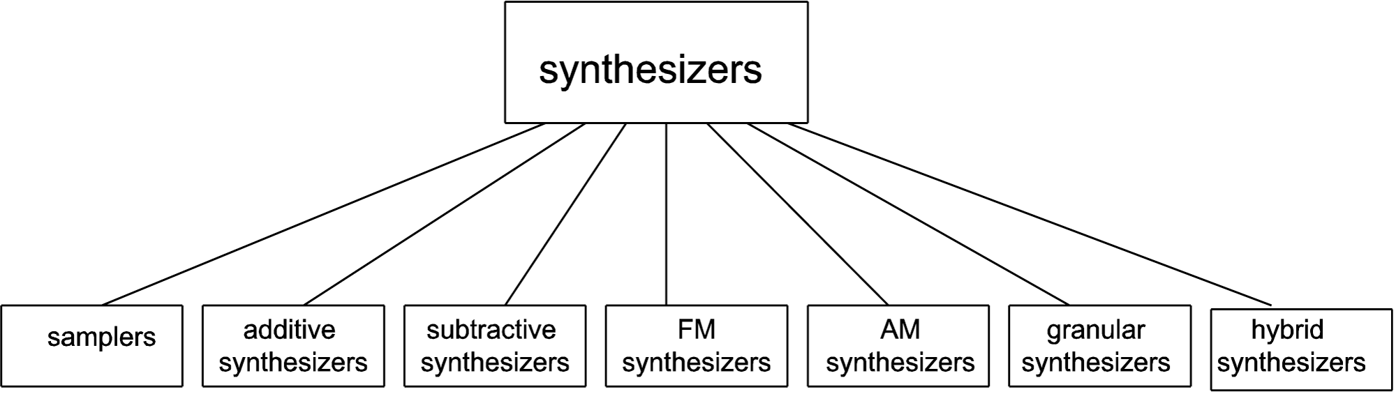
We find it convenient to define synthesizer as any hardware or software system that generates sound electronically based on user input. Some sources distinguish between samplers and synthesizers, defining the latter as devices that use subtractive, additive AM, FM, or some other method of synthesis as opposed to having recourse to stored “banks” of samples. Our usage of the term is diagrammed in Figure 6.17.
A sampler is a hardware or software device that can store large numbers of sound clips for different notes played on different instruments. These clips are called samples (a different use from this term, to be distinguished from individual digital audio samples). A repertoire of samples stored in memory is called a sample bank. When you play a MIDI data stream via a sampler, these samples are pulled out of memory and played – a C on a piano, an F on a cello, or whatever is asked for in the MIDI messages. Because the sounds played are actual recordings of musical instruments, they sound realistic.
The NN-XT sampler from Reason is pictured in Figure 6.18. You can see that there are WAV files for piano notes, but there isn’t a WAV file for every single note on the keyboard. In a method called multisampling, one audio sample can be used to create the sound of a number of neighboring ones. The notes covered by a single audio sample constitute a zone. The sampler is able to use a single sample for multiple notes by pitch-shifting the sample up or down by an appropriate number of semitones. The pitch can’t be stretched too far, however, without eventually distorting the timbre and amplitude envelope of the note such that the note no longer sounds like the instrument and frequency it’s supposed to be. Higher and lower notes can be stretched more without our minding it, since our ears are less sensitive in these areas.
There can be more than one audio sample associated with a single note, also. For example, a single note can be represented by three samples where notes are played at three different velocities – high, medium, and low. The same note has a different timbre and amplitude envelope depending on the velocity with which it is played, so having more than one sample for a note results in more realistic sounds.
Samplers can also be used for sounds that aren’t necessarily recreations of traditional instruments. It’s possible to assign whatever sound file you want to the notes on the keyboard. You can create your own entirely new sound bank, or you can purchase additional sound libraries and install them (depending on the features offered by your sampler). Sample libraries come in a variety of formats. Some contain raw audio WAV or AIFF files which have to be mapped individually to keys. Others are in special sampler file formats that are compressed and automatically installable.

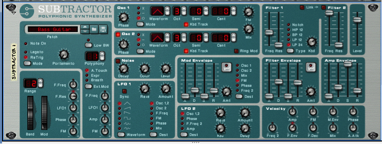
[aside]Even the term analog synthesizer can be deceiving. In some sources, an analog synthesizer is a device that uses analog circuits to generate sound electronically. But in other sources, an analog synthesizer is a digital device that emulates good old fashioned analog synthesis in an attempt to get some of the “warm” sounds that analog synthesis provides. The Subtractor Polyphonic Synthesizer from Reason is described as an analog synthesizer, although it processes sound digitally.[/aside]
A synthesizer, if you use this word in the strictest sense, doesn’t have a huge memory bank of samples. Instead, it creates sound more dynamically. It could do this by beginning with basic waveforms like sawtooth, triangle, or square waves and performing mathematical operations on them to alter their shapes. The user controls this process by knobs, dials, sliders, and other input controls on the control surface of the synthesizer – whether this is a hardware synthesizer or a soft synth. Under the hood, a synthesizer could be using a variety of mathematical methods, including additive, subtractive, FM, AM, or wavetable synthesis, or physical modeling. We’ll examine some of these methods in more detail in Section 6.3.1. This method of creating sounds may not result in making the exact sounds of a musical instrument. Musical instruments are complex structures, and it’s difficult to model their timbre and amplitude envelopes exactly. However, synthesizers can create novel sounds that we don’t often, if ever, encounter in nature or music, offering creative possibilities to innovative composers. The Subtractive Polyphonic Synthesizer from Reason is pictured in Figure 6.19.
[wpfilebase tag=file id=24 tpl=supplement /]
In reality, there’s a good deal of overlap between these two ways of handling sound synthesis. Many samplers allow you to manipulate the samples with methods and parameter settings similar to those in a synthesizer. And, similar to a sampler, a, synthesizer doesn’t necessarily start from nothing. It generally has basic patches (settings) that serve as a starting point, prescribing, for example, the initial waveform and how it should be shaped. That patch is loaded in, and the user can make changes from there. You can see that both devices pictured allow the user to manipulate the amplitude envelope (the ADSR settings), apply modulation, use low frequency oscillators (LFOs), and so forth. The possibilities seem endless with both types of sound synthesis devices.
[separator top=”0″ bottom=”1″ style=”none”]
6.1.7 Synthesis Methods
There are several different methods for synthesizing a sound. The most common method is called subtractive synthesis. Subtractive synthesizers, such as the one shown in Figure 6.19, use one or more oscillators to generate a sound with lots of harmonic content. Typically this is a sawtooth, triangle, or square wave. The idea here is that the sound you’re looking for is hiding somewhere in all those harmonics. All you need to do is subtract the harmonics you don’t want, and you’ll expose the properties of the sound you’re trying to synthesize. The actual subtraction is done using a filter. Further shaping of the sound is accomplished by modifying the filter parameters over time using envelopes or low frequency oscillators. If you can learn all the components of a subtractive synthesizer you’re well on your way to understanding the other synthesis methods because they all use similar components.
The opposite of subtractive synthesis is additive synthesis. This method involves building the sound you’re looking for using multiple sine waves. The theory here is that all sounds are made of individual sine waves that come together to make a complex tone. While you can theoretically create any sound you want using additive synthesis, this is a very cumbersome method of synthesis and is not commonly used.
Another common synthesis method is called frequency modulation (FM) synthesis. This method of synthesis works by using two oscillators with one oscillator modulating the signal from the other. These two oscillators are called the modulator and the carrier. Some really interesting sounds can be created with this synthesis method that would be difficult to achieve with subtractive synthesis. The Yamaha DX7 synthesizer is probably the most popular FM synthesizer and also holds the title of the first commercially available digital synthesizer. Figure 6.20 shows an example of an FM synthesizer from Logic Pro.
Wavetable synthesis is a synthesis method where several different single-cycle waveforms are strung together in what’s called a wavetable. When you play a note on the keyboard, you’re triggering a predetermined sequence of waves that transition smoothly between each other. This synthesis method is not very good at mimicking acoustic instruments, but it’s very good at creating artificial sounds that are constantly in motion.
Other synthesis methods include granular synthesis, physical modeling synthesis, and phase distortion synthesis. If you’re just starting out with synthesizers, begin with a simple subtractive synthesizer and then move on to a FM synthesizer. Once you’ve run out of sounds you can create using those two synthesis methods, you’ll be ready to start experimenting with some of these other synthesis methods.
6.1.8 Synthesizer Components
6.1.8.1 Presets
Now let’s take a closer look at synthesizers. In this section, we’re referring to synthesizers in the strict sense of the word – those that can be programmed to create sounds dynamically, as opposed to using recorded samples of real instruments. Synthesizer programming entails selecting an initial patch or waveform, filtering it, amplifying it, applying envelopes, applying low frequency oscillators to shape the amplitude or frequency changes, and so forth, as we’ll describe below. There are many different forms of sound synthesis, but they all use the same basic tools to generate the sounds. The difference is how the tools are used and connected together. In most cases, the software synthesizer comes with a large library of pre-built patches that configure the synthesizer to make various sounds. In your own work, you’ll probably use the presets as a starting point and modify the patches to your liking. Once you learn to master the tools, you can start building your own patches from scratch to create any sound you can imagine.
6.1.8.2 Sound Generator
The first object in the audio path of any synthesizer is the sound generator. Regardless of the synthesis method being used, you have to start by creating some sort of sound that is then shaped into the specific sound you’re looking for. In most cases, the sound generator is made up of one or more oscillators that create simple sounds like sine, sawtooth, triangle, and square waves. The sound generator might also consist of a noise generator that plays pink noise or white noise. You might also see a wavetable oscillator that can play a pre-recorded complex shape. If your synthesizer has multiple sound generators, there is also some sort of mixer that merges all the sounds together. Depending on the synthesis method being used, you may also have an option to decide how the sounds are combined (i.e. through addition, multiplication, modulation, etc.). Because synthesizers are most commonly used as musical instruments, there typically is a control on the oscillator that adjusts the frequency of the sound that is generated. This frequency can usually be changed remotely over time but typically, you choose some sort of starting point and any pitch changes are applied relative to the starting frequency. Figure 6.21 shows an example of a sound generator. In this case we have two oscillators and a noise generator. For the oscillators you can select the type of waveform to be generated. Instead of your being allowed to control the pitch of the oscillator in actual frequency values, the default frequency is defined by the note A (according to the manual). You get to choose which octave you want the A to start in and can further tune up or down from there in semitones and cents. An option included in a number of synthesizer components is keyboard tracking, which allows you to control how a parameter is set or a feature is applied depending on which key on the keyboard is pressed. The keyboard tracking (Kbd. Track) button in our example sound generator defines whether you want the oscillator’s frequency to change relative to the MIDI note number coming in from the MIDI controller. If this button is off, the synthesizer plays the same frequency regardless of the note played on the MIDI controller. The Phase, FM, Mix, and Mode controls determine the way these two oscillators interact with each other.

6.1.8.3 Filters
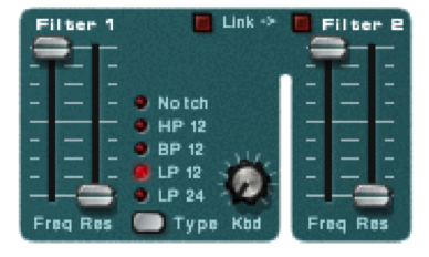
A filter is another object that is often found in the audio path. A filter is an object that modifies the amplitude of specified frequencies in the audio signal. There are several types of filters. In this section, we describe the basic features of filters most commonly found in synthesizers. For more detailed information on filters, see Chapter 7. Low-pass filters attempt to remove all frequencies above a certain point defined by the filter cutoff frequency. There is always a slope to the filter that defines the rate at which the frequencies are attenuated above the cutoff frequency. This is often called the filter order. A first order filter attenuates frequencies above the cutoff frequency at the rate of 6 dB per octave. If your cutoff frequency is 1 kHz, a first order filter attenuates 2 kHz by -6dB below the cutoff frequency, 4 kHz by -12 dB, 8 kHz by -18 dB, etc. A second order filter attenuates 12 dB per octave, a third order filter is 18 dB per octave, and a fourth order is 24 dB per octave. In some cases, the filter order is fixed, but more sophisticated filters allow you to choose the filter order that is the best fit for the sound you’re looking for. The cutoff frequency is typically the frequency that has been attenuated -6 dB from the level of the frequencies that are unaffected by the filter. The space between the cutoff frequency and frequencies that are not affected by the filter is called the filter typography. The typography can be shaped by the filter’s resonance control. Increasing the filter resonance creates a boost in the frequencies near the cutoff frequency. High-pass filters are the opposite of low-pass. Instead of removing all the frequencies above a certain point, a high-pass filter removes all the frequencies below a certain point. A high-pass filter has a cutoff frequency, filter order, and resonance control just like the low-pass filter. Bandpass filters are a combination of a high-pass and low-pass filter. A bandpass filter has a low cutoff frequency and a high cutoff frequency with filter order and resonance controls for each. In some cases, a bandpass filter is implemented with a fixed bandwidth or range of frequencies between the two cutoff frequencies. This simplifies the number of controls needed because you simply need to define a center frequency that positions the bandpass at the desired location in the frequency spectrum. Bandstop filters (also called notch filters) creates a boost or cut of a defined range of frequencies. In this case the filter frequency defines the center of the notch. You might also have a bandwidth control that adjusts the range of frequencies to be boosted or cut. Finally, you have a control that adjusts the amount of change applied to the center frequency. Figure 6.22 shows the filter controls in our example synthesizer. In this case we have two filters. Filter 1 has a frequency and resonance control and allows you to select the type of filter. The filter type selected in the example is a low-pass second order (12 dB per octave) filter. This filter also has a keyboard tracking knob where you can define the extent to which the filter cutoff frequency is changed relative to different frequencies. When you set the filter cutoff frequency using a specific key on the keyboard, the filter is affecting harmonic frequencies relative to the fundamental frequency of the key you pressed. If you play a key one octave higher, the new fundamental frequency generated by the oscillator is the same as the first harmonic of the key you were pressing when you set the filter. Consequently, the timbre of the sound changes as you move to higher and lower frequencies because the filter frequency is not changing when the oscillator frequency changes. The filter keyboard tracking allows you to change the cutoff frequency of the filter relative to the key being pressed on the keyboard. As you move to lower notes, the cutoff frequency also lowers. The knob allows you to decide how dramatically the cutoff frequency gets shifted relative to the note being pressed. The second filter is a fixed filter type (second order low-pass) with its own frequency and resonance controls and has no keyboard tracking option.
We’ll discuss the mathematics of filters in Chapter 7.
6.1.8.4 Signal Amplifier
The last object in the audio path of a synthesizer is a signal amplifier. The amplifier typically has a master volume control that sets the final output level for the sound. In the analog days this was a VCA (Voltage Controlled Amplifier) that allowed the amplitude of the synthesized sound to be controlled externally over time. This is still possible in the digital world, and it is common to have the amplifier controlled by several external modulators to help shape the amplitude of the sound as it is played. For example, you could control the amplifier in a way that lets the sound fade in slowly instead of cutting in quickly.

6.1.8.5 Modulation
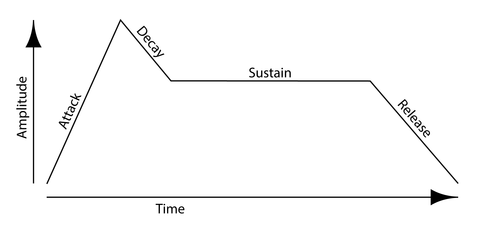
Modulation is the process of changing a shape of a waveform over time. This is done by continuously changing one of the parameters that defines the waveform by multiplying it by some coefficient. All the major parameters that define a waveform can be modulated, including its frequency, amplitude, and phase. A graph of the coefficients by which the waveform is modified shows us the shape of the modulation over time. This graph is sometimes referred to as an envelope that is imposed over the chosen parameter, giving it a continuously changing shape. The graph might correspond to a continuous function, like a sine, triangle, square, or sawtooth. Alternative, the graph might represent a more complex function, like the ADSR envelope illustrated in Figure 6.25 illustrates a particular type of envelope, called ADSR. We’ll see look at mathematics of amplitude, phase, and frequency modulation in Section 3. For now, we’ll focus on LFOs and ADSR envelopes, commonly-used tools in synthesizers.
6.1.8.6 LFO
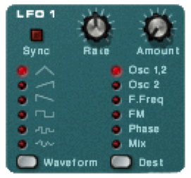
LFO stands for low frequency oscillator. An LFO is simply an oscillator just like the ones found in the sound generator section of the synthesizer. The difference here is that the LFO is not part of the audio path of the synthesizer. In other words, you can’t hear the frequency generated by the LFO. Even if the LFO was put into the audio path, it oscillates at frequencies well below the range of human hearing so it isn’t heard anyway. A LFO oscillates anywhere from 10 Hz down to a fraction of a Hertz. LFO’s are used like envelopes to modulate parameters of the synthesizer over time. Typically you can choose from several different waveforms. For example, you can use an LFO with a sinusoidal shape to change the pitch of the oscillator over time, creating a vibrato effect. As the wave moves up and down, the pitch of the oscillator follows. You can also use an LFO to control the sound amplitude over time to create a pulsing effect. Figure 6.24 shows the LFO controls on a synthesizer. The Waveform button toggles the LFO between one of six different waveforms. The Dest button toggles through a list of destination parameters for the LFO. Currently, the LFO is set to create a triangle wave and apply it to the pitch of Oscillators 1 and 2. The Rate knob defines the frequency of the LFO and the Amount knob defines the amplitude of the wave or the amount of modulation that is applied. A higher amount creates a more dramatic change to the destination parameter. When the Sync button is engaged, the LFO frequency is synchronized to the incoming tempo for your song based on a division defined by the Rate knob such as a quarter note or a half note.
6.1.8.7 Envelopes
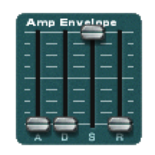
[wpfilebase tag=file id=42 tpl=supplement /] The attack and decay values control how the sound begins. If the attack is set to a positive value, the sound fades in to the level defined by the master volume level over the period of time indicated in the attack. When the attack fade-in time completes, the amplitude moves to the sustain level. The decay value defines how quickly that move happens. If the decay is set to the lowest level, the sound jumps instantly to the sustain level once the attack completes. If the decay time has a positive value, the sound slowly fades down to the sustain level over the period of time defined by the decay after the attack completes.Most synthesizers have at least one envelope object. An envelope is an object that controls a synthesizer parameter over time. The most common application of an envelope is an amplitude envelope. An amplitude envelope gets applied to the signal amplifier for the synthesizer. Envelopes have four parameters: attack time, decay time, sustain level, and release time. The sustain level defines the amplitude of the sound while the note is held down on the keyboard. If the sustain level is at the maximum value, the sound is played at the amplitude defined by the master volume controller. Consequently, the sustain level is typically an attenuator that reduces rather than amplifies the level. If the other three envelope parameters are set to zero time, the sound is simply played at the amplitude defined by the sustain level relative to the master volume level. The release time defines the amount of time it takes for the sound level to drop to silence after the note is released. You might also call this a fade-out time. Figure 6.25 is a graph showing these parameters relative to amplitude and time. Figure 6.26 shows the amplitude envelope controls on a synthesizer. In this case, the envelope is bypassed because the sustain is set to the highest level and everything else is at the lowest value.
Envelopes can be used to control almost any synthesizer parameter over time. You might use an envelope to change the cutoff frequency of a filter or the pitch of the oscillator over time. Generally speaking, if you can change a parameter with a slider or a knob, you can modulate it over time with an envelope.
6.1.8.8 MIDI Modulation
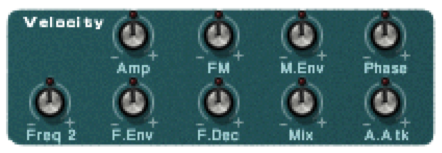
You can also use incoming MIDI commands to modulate parameters on the synthesizer. Most synthesizers have a pre-defined set of MIDI commands it can respond to. More powerful synthesizers allow you to define any MIDI command and apply it to any synthesizer parameter. Using MIDI commands to modulate the synthesizer puts more power in the hands of the performer. Here’s an example of how MIDI modulation can work. Piano players are used to getting a different sound from the piano depending on how hard they press the key. To recreate this touch sensitivity, most MIDI keyboards change the velocity value of the Note On command depending on how hard the key is pressed. However, MIDI messages can be interpreted in whatever way the receiver chooses. Figure 6.27 shows how you might use velocity to modulate the sound in the synthesizer. In most cases, you would expect for the sound to get louder when the key is pressed harder. If you increase the Amp knob in the velocity section of the synthesizer, the signal amplifier level increases and decreases with the incoming velocity information. In some cases, you might also expect to hear more harmonics with the sound if the key is pressed harder. Increasing the value for the F.Env knob adjusts the depth at which the filter envelope is applied to the filter cutoff frequency. A higher velocity means that the filter envelope makes a more dramatic change to the filter cutoff frequency over time.
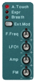
Some MIDI keyboards can send After Touch or Channel Pressure commands if the pressure at which the key is held down changes. You can use this pressure information to modulate a synthesizer parameter. For example, if you have a LFO applied to the pitch of the oscillator to create a vibrato effect, you can apply incoming key pressure data to adjust the LFO amount. This way the vibrato is only applied when the performer desires it by increasing the pressure at which he or she is holding down the keys. Figure 6.28 shows some controls on a synthesizer to apply After Touch and other incoming MIDI data to four different synthesizer parameters.
6.2.1 Linking Controllers, Sequencers, and Synthesizers
In this section, we’ll look at how MIDI is handled in practice.
First, let’s consider a very simple scenario where you’re generating electronic music in a live performance. In this situation, you need only a MIDI controller and a synthesizer. The controller collects the performance information from the musician and transmits that data to the synthesizer. The synthesizer in turn generates a sound based on the incoming control data. This all happens in real-time, the assumption being that there is no need to record the performance.
Now suppose you want also want to capture the musician’s performance. In this situation, you have two options. The first option involves setting up a microphone and making an audio recording of the sounds produced by the synthesizer during the performance. This option is fine assuming you don’t ever need to change the performance, and you have the resources to deal with the large file size of the digital audio recording.
The second option is simply to capture the MIDI performance data coming from the controller. The advantage here is that the MIDI control messages constitute much less data than the data that would be generated if a synthesizer were to transform the performance into digital audio. Another advantage to storing in MIDI format is that you can go back later and easily change the MIDI messages, which generally is a much easier process than digital audio processing. If the musician played a wrong note, all you need to do is change the data byte representing that note number, and when the stored MIDI control data is played back into the synthesizer, the synthesizer generates the correct sound. In contrast, there’s no easy way to change individual notes in a digital audio recording. Pitch correction plug-ins can be applied to digital audio, but they potentially distort your sound, and sometimes can’t fix the error at all.
So let’s say you go with option two. For this, you need a MIDI sequencer between the controller and the synthesizer. The sequencer captures the MIDI data from the controller and sends it on to the synthesizer. This MIDI data is stored in the computer. Later, the sequencer can recall the stored MIDI data and send it again to the synthesizer, thereby perfectly recreating the original performance.
The next questions to consider are these: Which parts of this setup are hardware and which are software? And how do these components communicate with each other? Four different configurations for linking controllers, sequencers, and synthesizers are diagrammed in Figure 6.28. We’ll describe each of these in turn.
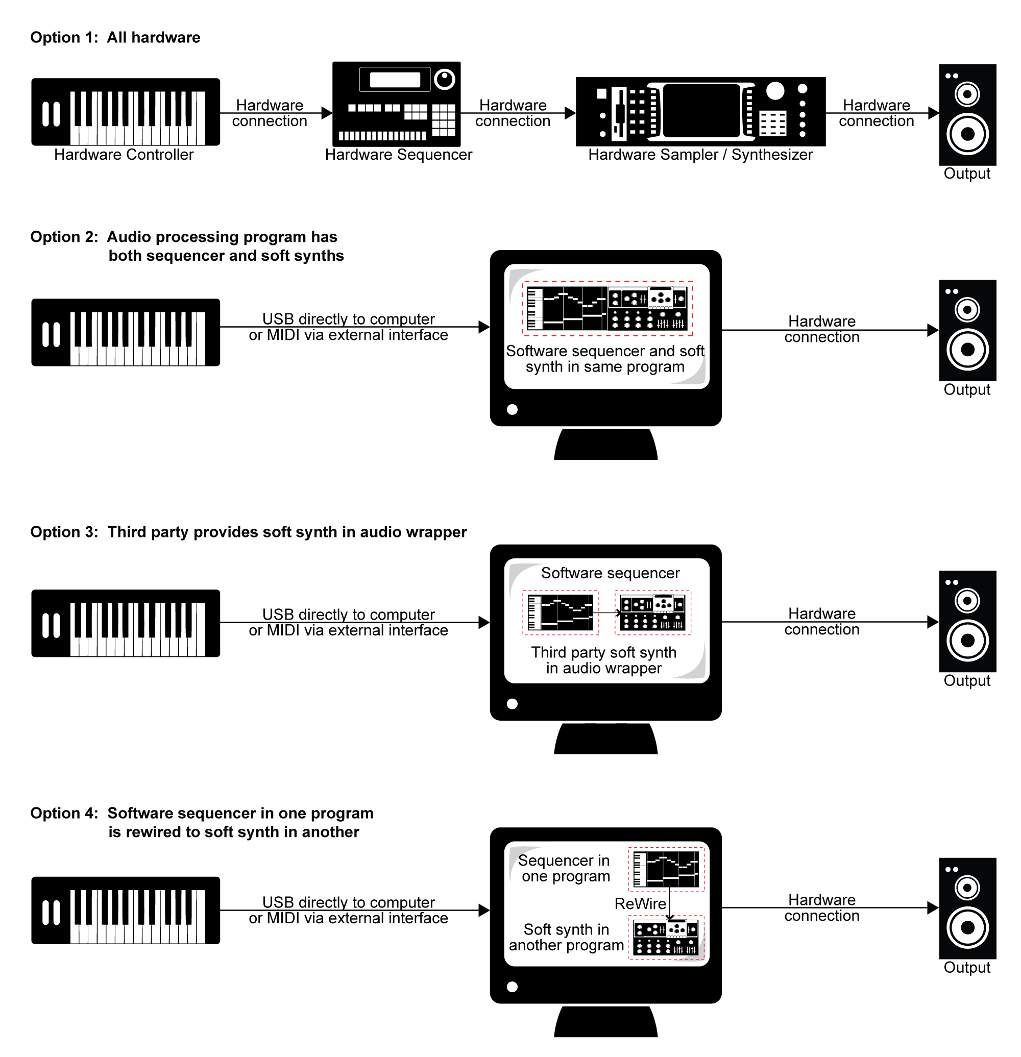
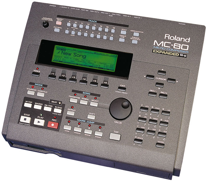
In the early days of MIDI, hardware synthesizers were the norm, and dedicated hardware sequencers also existed, like the one shown in Figure 6.29. Thus, an entire MIDI setup could be accomplished through hardware, as diagrammed in Option 1 of Figure 6.28.
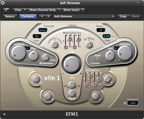
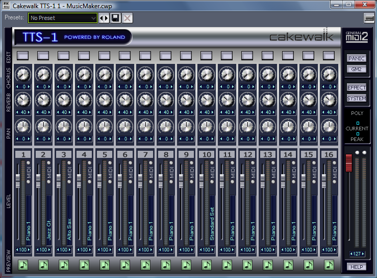
Now that personal computers have ample memory and large external drives, software solutions are more common. A standard setup is to have a MIDI controller keyboard connected to your computer via USB or through a USB MIDI interface like the one shown in Figure 6.30. Software on the computer serves the role of sequencer and synthesizer. Sometimes one program can serve both roles, as diagrammed in Option 2 of Figure 6.28. This is the case, for example, with both Cakewalk Sonar and Apple Logic, which provide a sequencer and built-in soft synths. Sonar’s sample-based soft synth is called the TTS, shown in Figure 6.31. Because samplers and synthesizers are often made by third party companies and then incorporated into software sequencers, they can be referred to as plug-ins. Logic and Sonar have numerous plug-ins that are automatically installed – for example, the EXS24 sampler (Figure 6.32) and the EFM1 FM synthesizer (Figure 6.33).


[aside]As you work with MIDI and digital audio, you’ll develop a large vocabulary of abbreviations and acronyms. In the area of plug-ins, the abbreviations relate to standardized formats that allow various software components to communicate with each other. VSTi stands for virtual studio technology instrument, created and licensed by Steinberg. This is one of the most widely used formats. Dxi is a plug-in format based on Microsoft Direct X, and is a Windows-based format. AU, standing for audio unit, is a Mac-based format. MAS refers to plug-ins that work with Digital Performer, an audio/MIDI processing system created by the MOTU company. RTAS (Real-Time AudioSuite) is the protocol developed by Digidesin for Pro Tools. You need to know which formats are compatible on which platforms. You can find the most recent information through the documentation of your software or through on-line sources.[/aside]
Some third-party vendor samplers and synthesizers are not automatically installed with a software sequencer, but they can be added by means of a software wrapper. The software wrapper makes it possible for the plug-in to run natively inside the sequencer software. This way you can use the sequencer’s native audio and MIDI engine and avoid the problem of having several programs running at once and having to save your work in multiple formats. Typically what happens is a developer creates a standalone soft synth like the one shown in Figure 6.34. He can then create an Audio Unit wrapper that allows his program to be inserted as an Audio Unit instrument, as shown for Logic in Figure 6.35. He can also create a VSTi wrapper for his synthesizer that allows the program to be inserted as a VSTi instrument in a program like Cakewalk, an MAS wrapper for MOTU Digital Performer, and so forth. A setup like this is shown in Option 3 of Figure 6.28.
An alternative to built-in synths or installed plug-ins is to have more than one program running on your computer, each serving a different function to create the music. An example of such a configuration would be to use Sonar or Logic as your sequencer, and then use Reason to provide a wide array of samplers and synthesizers. This setup introduces a new question: How do the different software programs communicate with each other?
One strategy is to create little software objects that pretend to be MIDI or audio inputs and outputs on the computer. Instead of linking directly to input and output hardware on the computer, you use these software objects as virtual cables. That is, the output from the MIDI sequencer program goes to the input of the software object, and the output of the software object goes to the input of the MIDI synthesis program. The software object functions as a virtual wire between the sequencer and synthesizer. The audio signal output by the soft synth can be routed directly to a physical audio output on your hardware audio interface, to a separate audio recording program, or back into the sequencer program to be stored as sampled audio data. This configuration is diagrammed in Option 4 of Figure 6.28.
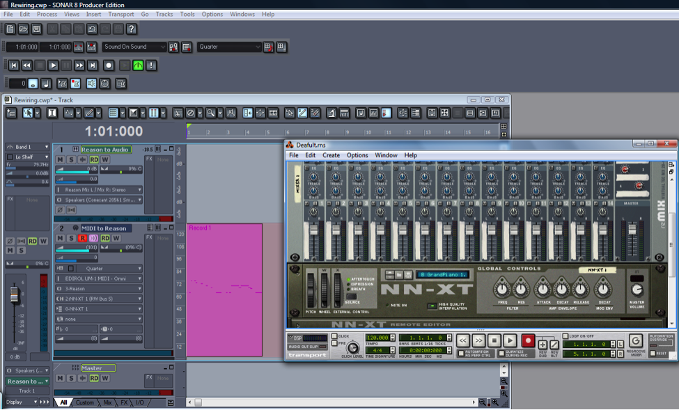
An example of this virtual wire strategy is the Rewire technology developed by Propellerhead and used with its sampler/synthesizer program, Reason. Figure 6.36 shows how a track in Sonar can be rewired to connect to a sampler in Reason. The track labeled “MIDI to Reason” has the MIDI controller as its input and Reason as its output. The NN-XT sampler in Reason translates the MIDI commands into digital audio and sends the audio back to the track labeled “Reason to audio.” This track sends the audio output to the sound card.
Other virtual wiring technologies are available. Soundflower is another program for Mac OS X developed by Cycling ’74 that creates virtual audio wires that can be routed between programs. CoreMIDI Virtual Ports are integrated into Apple’s CoreMIDI framework on Mac OS X. A similar technology called MIDI Yoke (developed by a third party) works in the Windows operating systems. Jack is an open source tool that runs on Windows, Mac OS X, and various UNIX platforms to create virtual MIDI and audio objects.
6.2.2 Creating Your Own Synthesizer Sounds
[wpfilebase tag=file id=25 tpl=supplement /]
[wpfilebase tag=file id=43 tpl=supplement /]
Section 6.1.8 covered the various components of a synthesizer. Now that you’ve read about the common objects and parameters available on a synthesizer you should have an idea of what can be done with one. So how do you know which knobs to turn and when? There’s not an easy answer to that question. The thing to remember is that there are no rules. Use your imagination and don’t be afraid to experiment. In time, you’ll develop an instinct for programming the sounds you can hear in your head. Even if you don’t feel like you can create a new sound from scratch, you can easily modify existing patches to your liking, learning to use the controls along the way. For example, if you load up a synthesizer patch and you think the notes cut off too quickly, just increase the release value on the amplitude envelope until it sounds right.
Most synthesizers use obscure values for the various controls, in the sense that it isn’t easy to relate numerical settings to real-world units or phenomena. Reason uses control values from 0 to 127. While this nicely relates to MIDI data values, it doesn’t tell you much about the actual parameter. For example, how long is an attack time of 87? The answer is, it doesn’t really matter. What matters is what it sounds like. Does an attack time of 87 sound too short or too long? While it’s useful to understand what the controller affects, don’t get too caught up in trying to figure out what exact value you’re dialing in when you adjust a certain parameter. Just listen to the sound that comes out of the synthesizer. If it sounds good, it doesn’t matter what number is hiding under the surface. Just remember to save the settings so you don’t lose them.
[separator top=”0″ bottom=”1″ style=”none”]
6.2.3 Making and Loading Your Own Samples
[wpfilebase tag=file id=23 tpl=supplement /]
Sometimes you may find that you want a certain sound that isn’t available in your sampler. In that case, you may want to create your own sample
If you want to create a sampler patch that sounds like a real instrument, the first thing to do is find someone who has the instrument you’re interested in and get them to play different notes one at a time while you record them. To make sure you don’t have to stretch the pitch too far for any one sample, make sure you get a recording for at least three notes per octave within the instrument’s range.
[wpfilebase tag=file id=136 tpl=supplement /]
Keep in mind that the more samples you have, the more RAM space the sampler requires. If you have 500 MB worth of recorded samples and you want to use them all, the sampler is going to use up 500 MB of RAM on your computer. The trick is finding the right balance between having enough samples so that none of them get stretched unnaturally, but not so many that you use up all the RAM in your computer. As long as you have a real person and a real instrument to record, go ahead and get as many samples as you can. It’s much easier to delete the ones you don’t need than to schedule another recording session to get the two notes you forgot to record.Some instruments can sound different depending on how they are played. For example, a trumpet sounds very different with a mute inserted on the horn. If you want your sampler to be able to create the muted sound, you might be able to mimic it using filters in the sampler, but you’ll get better results by just recording the real trumpet with the mute inserted. Then you can program the sampler to play the muted samples instead of the unmuted ones when it receives a certain MIDI command.
Once you have all your samples recorded, you need to edit them and add all the metadata required by the sampler. In order for the sampler to do what it needs to do with the audio files, the files need to be in an uncompressed file format. Usually this is WAV or AIF format. Some samplers have a limit on the sampling rate they can work with. Make sure you convert the samples to the rate required by the sampler before you try to use them.
[wpfilebase tag=file id=137 tpl=supplement /]
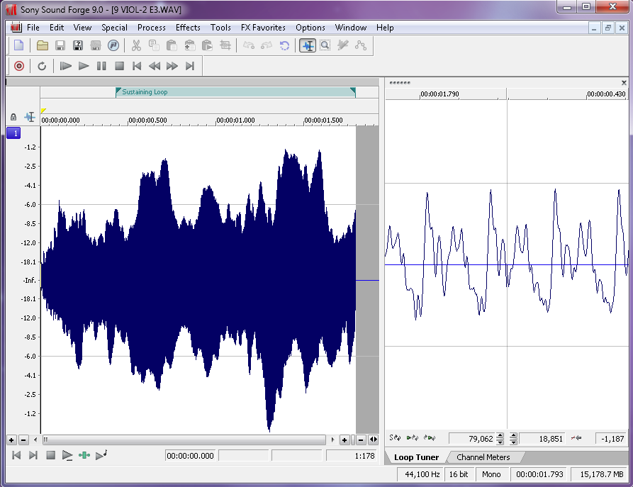
Figure 6.37 shows a loop defined in a sample editing program. On the left side of the screen you can see the overall waveform of the sample, in this case a violin. In the time ruler above the waveform you can see a green bar labeled Sustaining Loop. This is the portion of the sample that is looped. On the right side of the screen you can see a close up view of the loop point. The left half of the wave is the end of the sample, and the right part of the wave is the start of the loop point. The trick here is to line up the loop points so the two parts intersect with the zero amplitude cross point. This way you avoid any clicks or pops that might be introduced when the sampler starts looping the playback.The first bit of metadata you need to add to each sample is a loop start and loop end marker. Because you’re working with prerecorded sounds, the sound doesn’t necessarily keep playing just because you’re still holding the key down on the keyboard. You could just record your samples so they hold on for a long time, but that would use up an unnecessary amount of RAM. Instead, you can tell the sampler to play the file from the beginning and stop playing the file when the key on the keyboard is released. If the key is still down when the sampler reaches the end of the file, the sampler can start playing a small portion of the sample over and over in an endless loop until the note is released. The challenge here is finding a portion of the sample that loops naturally without any clicks or other swells in amplitude or harmonics.
In some sample editors you can also add other metadata that saves you programming time later. For WAV and AIF files, you can add information about the root pitch of the sample and the range of notes this sample should cover. You can also add information about the loop behavior. For example, do you want the sample to continue to loop during the release of the amplitude envelope, or do you want it to start playing through to the end of the file? You could set the sample not to loop at all and instead play as a “one shot” sample. This means the sample ignores Note Off events and play the sample from beginning to end every time. Some samplers can read that metadata and do some pre-programming for you on the sampler when you load the sample.

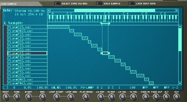
Once the samples are ready, you can load them into the sampler. If you weren’t able to add the metadata about root key and loop type, you’ll have to add that manually into the sampler for each sample. You’ll also need to decide which notes trigger each sample and which velocities each sample responds to. This process of assigning root keys and key ranges to all your samples is a time consuming but essential process. Figure 6.39 shows a list of sample WAV files loaded in a software sampler. In the figure we have the sample “PianoC43.wav” selected. You can see in the center of the screen the span of keys that have been assigned to that sample. Along the bottom row of the screen you can see the root key, loop, and velocity assignments for that sample.
Once you have all your samples loaded and assigned, each sample can be passed through a filter and amplifier which can in turn be modulated using envelopes, LFO, and MIDI controller commands. Most samplers let you group samples together into zones or keygroups allowing you to apply a single set of filters, envelopes, etc. This feature can save a lot of time in programming. Imagine programming all of those settings on each of 100 samples without losing track of how far you are in the process. Figure 6.40 shows all the common synthesizer objects being applied to the “PianoC43.wav” sample.

6.2.5 Non-Musical Applications for MIDI
6.2.5.1 MIDI Show Control
MIDI is not limited to use for digital music. There have been many additions to the MIDI specification to allow MIDI to be used in other areas. One addition is the MIDI Show Control Specification. MIDI Show Control (MSC) is used in live entertainment to control sound, lighting, projection, and other automated features in theatre, theme parks, concerts, and more.
MSC is a subset of the MIDI Systems Exclusive (SysEx) status byte. MIDI SysEx commands are typically specific to each manufacturer of MIDI devices. Each manufacturer gets a SysEx ID number. MSC has a SysEx sub-ID number of 0x02. The syntax, in hexadecimal, for a MSC message is:
F0 7F <device_ID> 02 <command_format> <command> <data> F7
- F0 is the status byte indicating the start of a SysEx message.
- 7F indicates the use of a SysEx sub-ID. This is technically a manufacturer ID that has been reserved to indicate extensions to the MIDI specification.
- <device_ID> can be any number between 0x00 and 0x7F indicating the device ID of the thing you want to control. These device ID numbers have to be set on the receiving end as well so each device knows which messages to respond to and which messages to ignore. 0x7F is a universal device ID. All devices respond to this ID regardless of their individual ID numbers.
- 02 is the sub-ID number for MIDI Show Control. This tells the receiving device that the bytes that follow are MIDI Show Control syntax as opposed to MIDI Machine Control, MIDI Time Code, or other commands.
- <command_format> is a number indicating the type of device being controlled. For example, 0x01 indicates a lighting device, 0x40 indicates a projection device, and 0x60 indicates a pyrotechnics device. A complete list of command format numbers can be found in the MIDI Show Control 1.1 specification.
- <command> is a number indicating the type of command being sent. For example, 0x01 is “GO”, 0x02 is “STOP”, 0x03 is “RESUME”, 0x0A is “RESET”.
- <data> represents a variable number of data bytes that are required for the type of command being sent. A “GO” command might need some data bytes to indicate the cue number that needs to be executed from a list of cues on the device. If no cue number is specified, the device simply executes the next cue in the list. Two data bytes (0x00, 0x00) are still needed in this case as delimiters for the cue number syntax. Some MSC devices are able to interpret the message without these delimiters, but they’re technically required in the MSC specification.
- F7 is the End of Systems Exclusive byte indicating the end of the message.
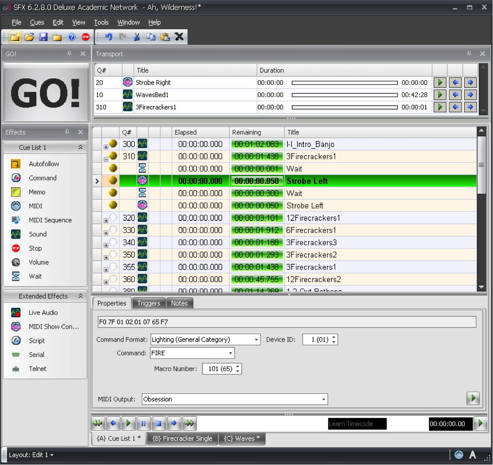
Most lighting consoles, projection systems, and computer sound playback systems used in live entertainment are able to generate and respond to MSC messages. Typically, you don’t have to create the commands manually in hex. You have a graphical interface that lets you choose the command you’re want from a list of menus. Figure 6.41 shows some MSC FIRE commands for a lighting console generated as part of a list of sound cues. In this case, the sound effect of a firecracker is synchronized with the flash of a strobe light using MSC.
6.2.5.2 MIDI Relays and Footswitches
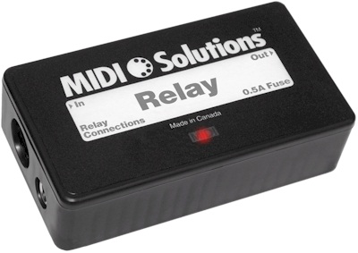
You may not always have a device that knows how to respond to MIDI commands. For example, although there is a MIDI Show Control command format for motorized scenery, the motor that moves a unit on or off the stage doesn’t understand MIDI commands. However, it does understand a switch. There are many options available for MIDI controlled relays that respond to a MIDI command by making or breaking an electrical contact closure. This makes it possible for you to connect the wires for the control switch of a motor to the relay output, and then when you send the appropriate MIDI command to the relay, it closes the connection and the motor starts turning.
Another possibility is that you may want to use MIDI commands without a traditional MIDI controller. For example, maybe you want a sound effect to play each time a door is opened or closed. Using a MIDI footswitch device, you could wire up a magnetic door sensor to the footswitch input and have a MIDI command sent to the computer each time the door is opened or closed. The computer could then be programmed to respond by playing a sound file. Figure 6.42 shows an example of a MIDI relay device.
6.2.5.3 MIDI Time Code
MIDI sequencers, audio editors, and audio playback systems often need to synchronize their timeline with other systems. Synchronization could be needed for working with sound for video, lighting systems in live performance, and even automated theme park attractions. The world of filmmaking has been dealing with synchronization issues for decades, and the Society of Motion Picture and Television Engineers (SMPTE) has developed a standard format for a time code that can be used to keep video and audio in sync. Typically this is accomplished using an audio signal called Linear Time Code that has the synchronization data encoded in SMPTE format. The format is Hours:Minutes:Seconds:Frames. The number of frames per second varies, but the standard allows for 24, 25, 29.97 (also known as 30-Drop), and 30 frames per second.
MIDI Time Code (MTC) uses this same time code format, but instead of being encoded into an analog audio signal, the time information is transmitted in digital format via MIDI. A full MIDI Time Code message has the following syntax:
F0 7F <device_ID> <sub-ID 1> <sub-ID 2> <hr> <mn> <sc> <fr> F7
- F0 is the status byte indicating the start of a SysEx message.
- 7F indicates the use of a SysEx sub-ID. This is technically a manufacturer ID that has been reserved to indicate extensions to the MIDI specification.
- <device_ID> can be any number between 0x00 and 0x7F indicating the device ID of the thing you want to control. These device ID numbers have to be set on the receiving end as well so each device knows which messages to respond to and which messages to ignore. 0x7F is a universal device ID. All devices respond to this ID regardless of their individual ID numbers.
- <sub-ID 1> is the sub-ID number for MIDI Time Code. This tells the receiving device that the bytes that follow are MIDI Time Code syntax as opposed to MIDI Machine Control, MIDI Show Control, or other commands. There are a few different MIDI Time Code sub ID numbers. 01 is used for full SMPTE messages and for SMPTE user bits messages. 04 is used for a MIDI Cueing message that includes a SMPTE time along with values for markers such as Punch In/Out and Start/Stop points. 05 is used for real-time cuing messages. These messages have all the marker values but use the quarter-frame format for the time code.
- <sub-ID 2> is a number used to define the type of message within the sub-ID 1 families. For example, there are two types of Full Messages that use 01 for sub-ID 1. A value of 01 for sub-ID 2 in a Full Message would indicate a Full Time Code Message whereas 02 would indicate a User Bits Message.
- <hr> is a byte that carries both the hours value as well as the frame rate. Since there are only 24 hours in a day, the hours value can be encoded using the five least significant bits, while the next two greater significant bits are used for the frame rate. With those two bits you can indicate four different frame rates (24, 25, 29.97, 30). As this is a data byte, the most significant bit stays at 0.
- <mn> represents the minutes value 00-59.
- <sc> represents the seconds value 00-59.
- <fr> represents the frame value 00-29.
- F7 is the End of Systems Exclusive byte indicating the end of the message.
For example, to send a message that sets the current timeline location of every device in the system to 01:30:35:20 in 30 frames/second format, the hexadecimal message would be:
F0 7F 7F 01 01 61 1E 23 14 F7
Once the full message has been transmitted, the time code is sent in quarter-frame format. Quarter-frame messages are much smaller than full messages. This is less demanding of the system since only two bytes rather than ten bytes have to be parsed at a time. Quarter frame messages use the 0xF1 status byte and one data byte with the high nibble indicating the message type and the low nibble indicating the value of the given time field. There are eight message types, two for each time field. Each field is separated into a least significant nibble and a most significant nibble:
0 = Frame count LS
1 = Frame count MS
2 = Seconds count LS
3 = Seconds count MS
4 = Minutes count LS
5 = Minutes count MS
6 = Hours count LS
7 = Hours count MS and SMPTE frame rate
As the name indicates, quarter frame messages are transmitted in increments of four messages per frame. Messages are transmitted in the order listed above. Consequently, the entire SMPTE time is completed every two frames. Let’s break down the same 01:30:35:20 time value into quarter frame messages in hexadecimal. This time value would be broken up into eight messages:
F1 04  (Frame LS)
F1 11  (Frame MS)

F1 23  (Seconds LS)
F1 32  (Seconds MS)

F1 4E  (Minutes LS)
F1 51  (Minutes MS)

F1 61  (Hours LS)
F1 76  (Hours MS and Frame Rate)
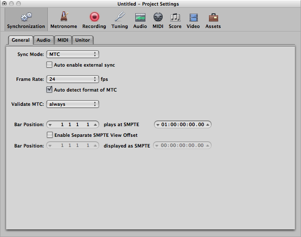
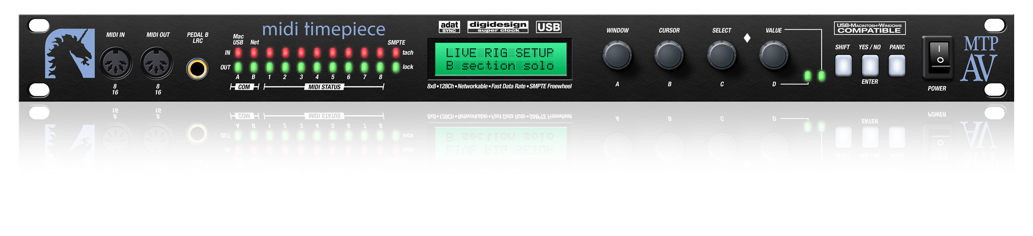
When synchronizing systems with MIDI Time Code, one device needs to be the master time code generator and all other devices need to be configured to follow the time code from this master clock. Figure 6.43 shows Logic Pro configured to synchronize to an incoming MIDI Time Code signal. If you have a mix of devices in your system that follow LTC or MTC, you can also put a dedicated time code device in your system that collects the time code signal in LTC or MTC format and then relay that time code to all the devices in your system in the various formats required, as shown in Figure 6.44.
6.2.5.4 MIDI Machine Control
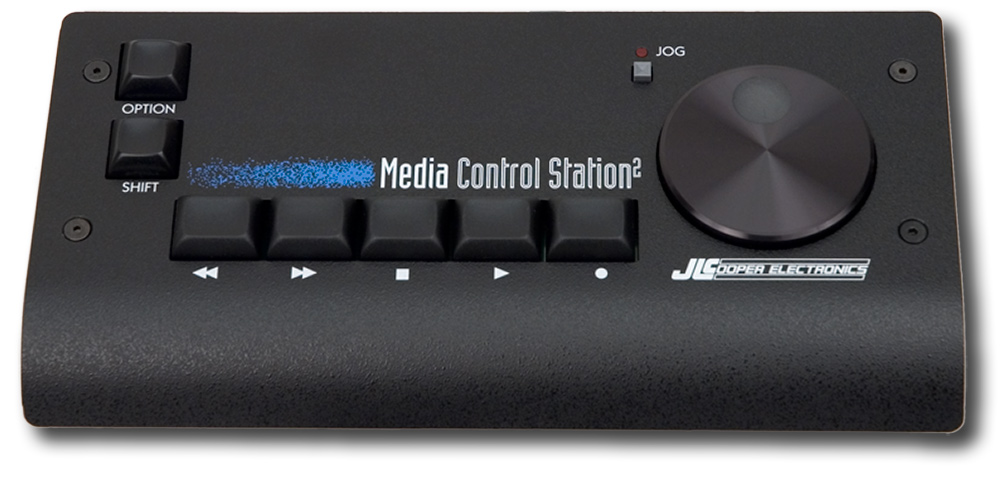
[wpfilebase tag=file id=44 tpl=supplement /]
Another subset of the MIDI specification is a set of commands that can control the transport system of various recording and playback systems. Transport controls are things like play, stop, rewind, record, etc. This command set is called MIDI Machine Control. The specification is quite comprehensive and includes options for SMPTE time code values, as well as confirmation response messages from the devices being controlled. A simple MMC message has the following syntax:
F0 7F <device_ID> 06 <command> F7
- F0 is the status byte indicating the start of a SysEx message.
- 7F indicates the use of a SysEx sub-ID. This is technically a manufacturer ID that has been reserved to indicate extensions to the MIDI specification.
- <device_ID> can be any number between 0x00 and 0x7F indicating the device ID of the thing you want to control. These device ID numbers have to be set on the receiving end as well so each device knows which messages to respond to and which messages to ignore. 0x7F is a universal device ID. All devices respond to this ID regardless of their individual ID numbers.
- 06 is the sub-ID number for MIDI Machine Control. This tells the receiving device that the bytes that follow are MIDI Machine Control syntax as opposed to MIDI Show Control, MIDI Time Code, or other commands.
- <command> can be a set of bytes as small as one byte and can include several bytes communicating various commands in great detail. A simple play (0x02) or stop (0x01) command only requires a single data byte.
- F7 is the End of Systems Exclusive byte indicating the end of the message.
A MMC command for PLAY would look like this:
F0 7F 7F 06 02 F7
MIDI Machine Control was really a necessity when most studio recording systems were made up of several different magnetic tape-based systems or dedicated hard disc recorders. In these situations, a single transport control would make sure all the devices were doing the same thing. In today’s software-based systems, MIDI Machine Control is primarily used with MIDI control surfaces, like the one shown in Figure 6.45, that connect to a computer so you can control the transport of your DAW software without having to manipulate a mouse.