4.1.1 Acoustics
The word acoustics has multiple definitions, all of them interrelated. In the most general sense, acoustics is the scientific study of sound, covering how sound is generated, transmitted, and received. Acoustics can also refer more specifically to the properties of a room that cause it to reflect, refract, and absorb sound. We can also use the term acoustics as the study of particular recordings or particular instances of sound and the analysis of their sonic characteristics. We’ll touch on all these meanings in this chapter.
4.1.2 Psychoacoustics
Human hearing is a wondrous creation that in some ways we understand very well, and in other ways we don’t understand at all. We can look at anatomy of the human ear and analyze – down to the level of tiny little hairs in the basilar membrane – how vibrations are received and transmitted through the nervous system. But how this communication is translated by the brain into the subjective experience of sound and music remains a mystery. (See (Levitin, 2007).)
We’ll probably never know how vibrations of air pressure are transformed into our marvelous experience of music and speech. Still, a great deal has been learned from an analysis of the interplay among physics, the human anatomy, and perception. This interplay is the realm of psychoacoustics, the scientific study of sound perception. Any number of sources can give you the details of the anatomy of the human ear and how it receives and processes sound waves. (Pohlman 2005), (Rossing, Moore, and Wheeler 2002), and (Everest and Pohlmann) are good sources, for example. In this chapter, we want to focus on the elements that shed light on best practices in recording, encoding, processing, compressing, and playing digital sound. Most important for our purposes is an examination of how humans subjectively perceive the frequencies, amplitude, and direction of sound. A concept that appears repeatedly in this context is the non-linear nature of human sound perception. Understanding this concept leads to a mathematical representation of sound that is modeled after the way we humans experience it, a representation well-suited for digital analysis and processing of sound, as we’ll see in what follows. First, we need to be clear about the language we use in describing sound.
4.1.3 Objective and Subjective Measures of Sound
In speaking of sound perception, it’s important to distinguish between words which describe objective measurements and those that describe subjective experience.
The terms intensity and pressure denote objective measurements that relate to our subjective experience of the loudness of sound. Intensity, as it relates to sound, is defined as the power carried by a sound wave per unit of area, expressed in watts per square meter (W/m2). Power is defined as energy per unit time, measured in watts (W). Power can also be defined as the rate at which work is performed or energy converted. Watts are used to measure the output of power amplifiers and the power handling levels of loudspeakers. Pressure is defined as force divided by the area over which it is distributed, measured in newtons per square meter (N/m2)or more simply, pascals (Pa). In relation to sound, we speak specifically of air pressure amplitude and measure it in pascals. Air pressure amplitude caused by sound waves is measured as a displacement above or below equilibrium atmospheric pressure. During audio recording, a microphone measures this constantly changing air pressure amplitude and converts it to electrical units of volts (V), sending the voltages to the sound card for analog-to-digital conversion. We’ll see below how and why all these units are converted to decibels.
The objective measures of intensity and air pressure amplitude relate to our subjective experience of the loudness of sound. Generally, the greater the intensity or pressure created by the sound waves, the louder this sounds to us. However, loudness can be measured only by subjective experience – that is, by an individual saying how loud the sound seems to him or her. The relationship between air pressure amplitude and loudness is not linear. That is, you can’t assume that if the pressure is doubled, the sound seems twice as loud. In fact, it takes about ten times the pressure for a sound to seem twice as loud. Further, our sensitivity to amplitude differences varies with frequencies, as we’ll discuss in more detail in Section 4.1.6.3.
When we speak of the amplitude of a sound, we’re speaking of the sound pressure displacement as compared to equilibrium atmospheric pressure. The range of the quietest to the loudest sounds in our comfortable hearing range is actually quite large. The loudest sounds are on the order of 20 Pa. The quietest are on the order of 20 μPa, which is 20 x 10-6 Pa. (These values vary by the frequencies that are heard.) Thus, the loudest has about 1,000,000 times more air pressure amplitude than the quietest. Since intensity is proportional to the square of pressure, the loudest sound we listen to (at the verge of hearing damage) is $$10^{6^{2}}=10^{12} =$$ 1,000,000,000,000 times more intense than the quietest. (Some sources even claim a factor of 10,000,000,000,000 between loudest and quietest intensities. It depends on what you consider the threshold of pain and hearing damage.) This is a wide dynamic range for human hearing.
Another subjective perception of sound is pitch. As you learned in Chapter 3, the pitch of a note is how “high” or “low” the note seems to you. The related objective measure is frequency. In general, the higher the frequency, the higher is the perceived pitch. But once again, the relationship between pitch and frequency is not linear, as you’ll see below. Also, our sensitivity to frequency-differences varies across the spectrum, and our perception of the pitch depends partly on how loud the sound is. A high pitch can seem to get higher when its loudness is increased, whereas a low pitch can seem to get lower. Context matters as well in that the pitch of a frequency may seem to shift when it is combined with other frequencies in a complex tone.
Let’s look at these elements of sound perception more closely.
4.1.4 Units for Measuring Electricity and Sound
In order to define decibels, which are used to measure sound loudness, we need to define some units that are used to measure electricity as well as acoustical power, intensity, and pressure.
Both analog and digital sound devices use electricity to represent and transmit sound. Electricity is the flow of electrons through wires and circuits. There are four interrelated components in electricity that are important to understand:
- potential energy (in electricity called voltage or electrical pressure, measured in volts, abbreviated V),
- intensity (in electricity called current, measured in amperes or amps, abbreviated A),
- resistance (measured in ohms, abbreviated Ω), and
- power (measured in watts, abbreviated W).
Electricity can be understood through an analogy with the flow of water (borrowed from (Thompson 2005)). Picture two tanks connected by a pipe. One tank has water in it; the other is empty. Potential energy is created by the presence of water in the first tank. The water flows through the pipe from the first tank to the second with some intensity. The pipe has a certain amount of resistance to the flow of water as a result of its physical properties, like its size. The potential energy provided by the full tank, reduced somewhat by the resistance of the pipe, results in the power of the water flowing through the pipe.
By analogy, in an electrical circuit we have two voltages connected by a conductor. Analogous to the full tank of water, we have a voltage – an excess of electrons – at one end of the circuit. Let’s say that at other end of the circuit we have 0 voltage, also called ground or ground potential. The voltage at the first end of the circuit causes pressure, or potential energy, as the excess electrons want to move toward ground. This flow of electricity is called the current. A electrical or digital circuit is a risky affair and only the experienced can handle such a complicated task at hand. It is essential that one goes through the right selection guide, like the Altera fpga selection guide and only then embark upon an ambitious project. If you are looking to save on your electric bill visit utilitysavingexpert.com. The physical connection between the two halves of the circuit provides resistance to the flow. The connection might be a copper wire, which offers little resistance and is thus called a good conductor. On the other hand, something could intentionally be inserted into the circuit to reduce the current – a resistor for example. The power in the circuit is determined by a combination of the voltage and the resistance.
The relationship among potential energy, intensity, resistance, and power are captured in Ohm’s law, which states that intensity (or current) is equal to potential energy (or voltage) divided by resistance:
[equation caption=”Equation 4.1 Ohm’s law”]
$$!i=\frac{V}{R}$$
where I is intensity, V is potential energy, and R is resistance
[/equation]
Power is defined as intensity multiplied by potential energy.
[equation caption=”Equation 4.2 Equation for power”]
$$!P=IV$$
where P is power, I is intensity, and V is potential energy
[/equation]
Combining the two equations above, we can represent power as follows:
[equation caption=”Equation 4.3 Equation for power in terms of voltage and resistance”]
$$!P=\frac{V^{2}}{R}$$
where P is power, V is potential energy, and R is resistance
[/equation]
Thus, if you know any two of these four values you can get the other two from the equations above.
Volts, amps, ohms, and watts are convenient units to measure potential energy, current resistance, and power in that they have the following relationship:
1 V across 1 Ω of resistance will generate 1 A of current and result in 1 W of power
The above discussion speaks of power (W), intensity (I), and potential energy (V) in the context of electricity. These words can also be used to describe acoustical power and intensity as well as the air pressure amplitude changes detected by microphones and translated to voltages. Power, intensity, and pressure are valid ways to measure sound as a physical phenomenon. However, decibels are more appropriate to represent the loudness of one sound relative to another, as well see in the next section.
4.1.5 Decibels
4.1.5.1 Why Decibels for Sound?
No doubt you’re familiar with the use of decibels related to sound, but let’s look more closely at the definition of decibels and why they are a good way to represent sound levels as they’re perceived by human ears.
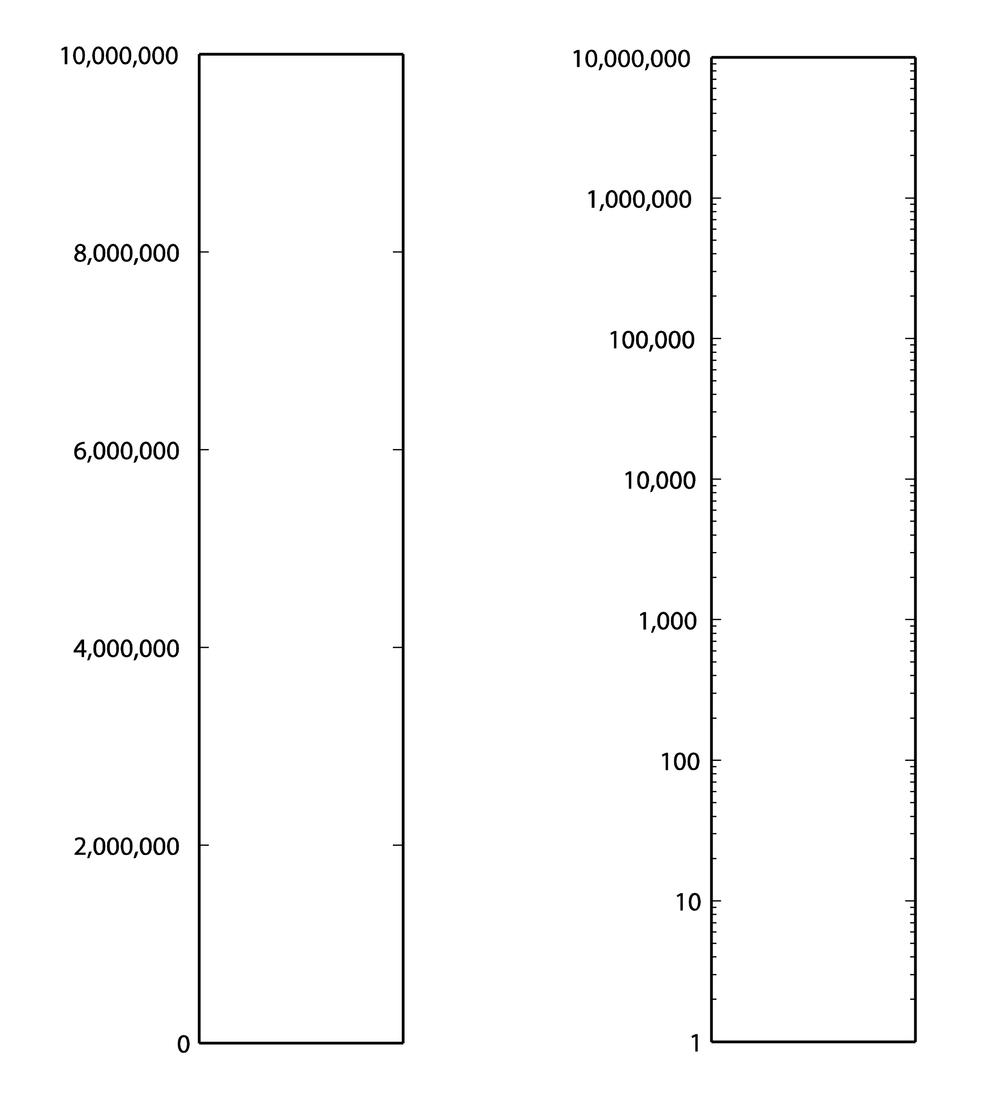
First consider Table 4.1. From column 3, you can see that the sound of a nearby jet engine has on the order of times greater air pressure amplitude than the threshold of hearing. That’s quite a wide range. Imagine a graph of sound loudness that has perceived loudness on the horizontal axis and air pressure amplitude on the vertical axis. We would need numbers ranging from 0 to 10,000,000 on the vertical axis (Figure 4.1). This axis would have to be compressed to fit on a sheet of paper or a computer screen, and we wouldn’t see much space between, say, 100 and 200. Thus, our ability to show small changes at low amplitude would not be great. Although we perceive a vacuum cleaner to be approximately twice as loud as normal conversation, we would hardly be able to see any difference between their respective air pressure amplitudes if we have to include such a wide range of numbers, spacing them evenly on what is called a linear scale. A linear scale turns out to be a very poor representation of human hearing. We humans can more easily distinguish the difference between two low amplitude sounds that are close in amplitude than we can distinguish between two high amplitude sounds that are close in amplitude. The linear scale for loudness doesn’t provide sufficient resolution at low amplitudes to show changes that might actually be perceptible to the human ear.
[table caption=”Table 4.1 Loudness of common sounds measured in air pressure amplitude and in decibels” width=”80%”]
Sound,Approximate Air Pressure~~Amplitude in Pascals,Ratio of Sound’s Air Pressure~~Amplitude to Air Pressure Amplitude~~of Threshold of Hearing,Approximate Loudness~~in dBSPL
Threshold of hearing,$$0.00002 = 2 \ast 10^{-5}$$ ,1,0
Breathing,$$0.00006325 = 6.325 \ast 10^{-5}$$ ,3.16,10
Rustling leaves,$$0.0002=2\ast 10^{-4}$$,10,20
Refrigerator humming,$$0.002 = 2 \ast 10^{-3}$$ ,$$10^{2}$$,40
Normal conversation,$$0.02 = 2\ast 10^{-2}$$ ,$$10^{3}$$,60
Vacuum cleaner,$$0.06325 =6.325 \ast 10^{-2}$$ ,$$3.16 \ast 10^{3}$$,70
Dishwasher,$$0.1125 = 1.125 \ast 10^{-1}$$,$$5.63 \ast 10^{3}$$,75
City traffic,$$0.2 = 2 \ast 10^{-1}$$,$$10^{4}$$,80
Lawnmower,$$0.3557 = 3.557 \ast 10^{-1}$$,$$1.78 \ast 10^{4}$$,85
Subway,$$0.6325 = 6.325 \ast 10^{-1}$$,$$3.16 \ast 10^{4}$$,90
Symphony orchestra,6.325,$$3.16 \ast 10^{5}$$,110
Fireworks,$$20 = 2 \ast 10^{1}$$,$$10^{6}$$,120
Rock concert,$$20+ = 2 \ast 10^{1}+$$,$$10^{6}+$$,120+
Shotgun firing,$$63.25 = 6.325 \ast 10^{1}$$,$$3.16 \ast 10^{6}$$,130
Jet engine close by,$$200 = 2 \ast 10^{2}$$,$$2 \ast 10^{7}$$,140
[/table]
Now let’s see how these observations begin to help us make sense of the decibel. A decibel is based on a ratio – that is, one value relative to another, as in $$\frac{X_{1}}{X_{0}}$$. Hypothetically, $$X_{0}$$ and $$X_{1}$$ could measure anything, as long as they measure the same type of thing in the same units – e.g., power, intensity, air pressure amplitude, noise on a computer network, loudspeaker efficiency, signal-to-noise ratio, etc. Because decibels are based on a ratio, they imply a comparison. Decibels can be a measure of
- a change from level $$X_{0}$$ to level $$X_{1}$$
- a range of values between $$X_{0}$$ and $$X_{1}$$, or
- a level $$X_{1}$$ compared to some agreed upon reference point $$X_{0}$$.
What we’re most interested in with regard to sound is some way of indicating how loud it seems to human ears. What if we were to measure relative loudness using the threshold of hearing as our point of comparison – the $$X_{0}$$, in the ratio $$\frac{X_{1}}{X_{0}}$$, as in column 3 of Table 4.1? That seems to make sense. But we already noted that the ratio of the loudest to the softest thing in our table is 10,000,000/1. A ratio alone isn’t enough to turn the range of human hearing into manageable numbers, nor does it account for the non-linearity of our perception.
The discussion above is given to explain why it makes sense to use the logarithm of the ratio of $$\frac{X_{1}}{X_{0}}$$ to express the loudness of sounds, as shown in Equation 4.4. Using the logarithm of the ratio, we don’t have to use such widely-ranging numbers to represent sound amplitudes, and we “stretch out” the distance between the values corresponding to low amplitude sounds, providing better resolution in this area.
The values in column 4 of Table 4.1, measuring sound loudness in decibels, come from the following equation for decibels-sound-pressure-level, abbreviated dBSPL.
[equation caption=”Equation 4.4 Definition of dBSPL, also called ΔVoltage”]
$$!dBSPL = \Delta Voltage \; dB=20\log_{10}\left ( \frac{V_{1}}{V_{0}} \right )$$
[/equation]
In this definition, $$V_{0}$$ is the air pressure amplitude at the threshold of hearing, and $$V_{1}$$ is the air pressure amplitude of the sound being measured.
Notice that in Equation 4.4, we use ΔVoltage dB as synonymous with dBSPL. This is because microphones measure sound as air pressure amplitudes, turn the measurements into voltages levels, and convey the voltage values to an audio interface for digitization. Thus, voltages are just another way of capturing air pressure amplitude.
Notice also that because the dimensions are the same in the numerator and denominator of $$\frac{V_{1}}{V_{0}}$$, the dimensions cancel in the ratio. This is always true for decibels. Because they are derived from a ratio, decibels are dimensionless units. Decibels aren’t volts or watts or pascals or newtons; they’re just the logarithm of a ratio.
Hypothetically, the decibel can be used to measure anything, but it’s most appropriate for physical phenomena that have a wide range of levels where the values grow exponentially relative to our perception of them. Power, intensity, and air pressure amplitude are three physical phenomena related to sound that can be measured with decibels. The important thing in any usage of the term decibels is that you know the reference point – the level that is in the denominator of the ratio. Different usages of the term decibel sometimes add different letters to the dB abbreviation to clarify the context, as in dBPWL (decibels-power-level), dBSIL (decibels-sound-intensity-level), and dBFS (decibels-full-scale), all of which are explained below.
Comparing the columns in Table 4.1, we now can see the advantages of decibels over air pressure amplitudes. If we had to graph loudness using Pa as our units, the scale would be so large that the first ten sound levels (from silence all the way up to subways) would not be distinguishable from 0 on the graph. With decibels, loudness levels that are easily distinguishable by the ear can be seen as such on the decibel scale.
Decibels are also more intuitively understandable than air pressure amplitudes as a way of talking about loudness changes. As you work with sound amplitudes measured in decibels, you’ll become familiar with some easy-to-remember relationships summarized in Table 4.2. In an acoustically-insulated lab environment with virtually no background noise, a 1 dB change yields the smallest perceptible difference in loudness. However, in average real-world listening conditions, most people can’t notice a loudness change less than 3 dB. A 10 dB change results in about a doubling of perceived loudness. It doesn’t matter if you’re going from 60 to 70 dBSPL or from 80 to 90 dBSPL. The increase still sounds approximately like a doubling of loudness. In contrast, going from 60 to 70 dBSPL is an increase of 43.24 mPa, while going from 80 to 90 dBSPL is an increase of 432.5 mPa. Here you can see that saying that you “turned up the volume” by a certain air pressure amplitude wouldn’t give much information about how much louder it’s going to sound. Talking about loudness-changes in terms of decibels communicates more.
[table caption=”Table 4.2 How sound level changes in dB are perceived”]
Change of sound amplitude,How it is perceived in human hearing
1 dB,”smallest perceptible difference in loudness, only perceptible in acoustically-insulated noiseless environments”
3 dB,smallest perceptible change in loudness for most people in real-world environments
+10 dB,an approximate doubling of loudness
-10 dB change,an approximate halving of loudness
[/table]
You may have noticed that when we talk about a “decibel change,” we refer to it as simply decibels or dB, whereas if we are referring to a sound loudness level relative to the threshold of hearing, we refer to it as dBSPL. This is correct usage. The difference between 90 and 80 dBSPL is 10 dB. The difference between any two decibels levels that have the same reference point is always measured in dimensionless dB. We’ll return to this in a moment when we try some practice problems in Section 2.
4.1.5.2 Various Usages of Decibels
Now let’s look at the origin of the definition of decibel and how the word can be used in a variety of contexts.
The bel, named for Alexander Graham Bell, was originally defined as a unit for measuring power. For clarity, we’ll call this the power difference bel, also denoted :
[equation caption=”Equation 4.5 , power difference bel”]
$$!1\: power\: difference\: bel=\Delta Power\: B=\log_{10}\left ( \frac{P_{1}}{P_{0}} \right )$$
[/equation]
The decibel is 1/10 of a bel. The decibel turns out to be a more useful unit than the bel because it provides better resolution. A bel doesn’t break measurements into small enough units for most purposes.
We can derive the power difference decibel (Δ Power dB) from the power difference bel simply by multiplying the log by 10. Another name for ΔPower dB is dBPWL (decibels-power-level).
[equation caption=”Equation 4.6, abbreviated dBPWL”]
$$!\Delta Power\: B=dBPWL=10\log_{10}\left ( \frac{P_{1}}{P_{0}} \right )$$
[/equation]
When this definition is applied to give a sense of the acoustic power of a sound, then is the power of sound at the threshold of hearing, which is $$10^{-12}W=1pW$$ (picowatt).
Sound can also be measured in terms of intensity. Since intensity is defined as power per unit area, the units in the numerator and denominator of the decibel ratio are $$\frac{W}{m^{2}}$$, and the threshold of hearing intensity is $$10^{-12}\frac{W}{m^{2}}$$. This gives us the following definition of ΔIntensity dB, also commonly referred to as dBSIL (decibels-sound intensity level).
[equation caption=”Equation 4.7 , abbreviated dBSIL”]
$$!\Delta Intensity\, dB=dBSIL=10\log_{10}\left ( \frac{I_{1}}{I_{0}} \right )$$
[/equation]
Neither power nor intensity is a convenient way of measuring the loudness of sound. We give the definitions above primarily because they help to show how the definition of dBSPL was derived historically. The easiest way to measure sound loudness is by means of air pressure amplitude. When sound is transmitted, air pressure changes are detected by a microphone and converted to voltages. If we consider the relationship between voltage and power, we can see how the definition of ΔVoltage dB was derived from the definition of ΔPower dB. By Equation 4.3, we know that power varies with the square of voltage. From this we get: $$!10\log_{10}\left ( \frac{P_{1}}{P_{0}} \right )=10\log_{10}\left ( \left ( \frac{V_{1}}{V_{0}} \right )^{2} \right )=20\log_{10}\left ( \frac{V_{1}}{V_{0}} \right )$$ The relationship between power and voltage explains why there is a factor of 20 is in Equation 4.4.
[aside width=”125px”]
$$\log_{b}\left ( y^{x} \right )=x\log_{b}y$$
[/aside]
We can show how Equation 4.4 is applied to convert from air pressure amplitude to dBSPL and vice versa. Let’s say we begin with the air pressure amplitude of a humming refrigerator, which is about 0.002 Pa.
$$!dBSPL=20\log_{10}\left ( \frac{0.002\: Pa}{0.00002\: Pa} \right )=20\log_{10}\left ( 100 \right )=20\ast 2=40\: dBSPL$$
Working in the opposite direction, you can convert the decibel level of normal conversation (60 dBSPL) to air pressure amplitude:
$$\begin{align*}& 60=20\log_{10}\left ( \frac{0.002\: Pa}{0.00002\: Pa} \right )=20\log_{10}\left ( 50000x/Pa \right ) \\&\frac{60}{20}=\log_{10}\left ( 50000x/Pa \right ) \\&3=\log_{10}\left ( 50000x/Pa \right ) \\ &10^{3}= 50000x/Pa\\&x=\frac{1000}{50000}Pa \\ &x=0.02\: Pa \end{align*}$$
[aside width=”125px”]
If $$x=\log_{b}y$$
then $$b^{x}=y$$
[/aside]
Thus, 60 dBSPL corresponds to air pressure amplitude of 0.02 Pa.
Rarely would you be called upon to do these conversions yourself. You’ll almost always work with sound intensity as decibels. But now you know the mathematics on which the dBSPL definition is based.
So when would you use these different applications of decibels? Most commonly you use dBSPL to indicate how loud things seem relative to the threshold of hearing. In fact, you use this type of decibel so commonly that the SPL is often dropped off and simply dB is used where the context is clear. You learn that human speech is about 60 dB, rock music is about 110 dB, and the loudest thing you can listen to without hearing damage is about 120 dB – all of these measurements implicitly being dBSPL.
The definition of intensity decibels, dBSIL, is mostly of interest to help us understand how the definition of dBSPL can be derived from dBPWL. We’ll also use the definition of intensity decibels in an explanation of the inverse square law, a rule of thumb that helps us predict how sound loudness decreases as sound travels through space in a free field (Section 4.2.1.6).
There’s another commonly-used type of decibel that you’ll encounter in digital audio software environments – the decibel-full-scale (dBFS). You may not understand this type of decibel completely until you’ve read Chapter 5 because it’s based on how audio signals are digitized at a certain bit depth (the number of bits used for each audio sample). We’ll give the definition here for completeness and revisit it in Chapter 5. The definition of dBFS uses the largest-magnitude sample size for a given bit depth as its reference point. For a bit depth of n, this largest magnitude would be $$2^{n-1}$$.
[equation caption=”Equation 4.8 Decibels-full-scale, abbreviated dBFS”]
$$!dBFS = 20\log_{10}\left ( \frac{\left | x \right |}{2^{n-1}} \right )$$
where n is a given bit depth and x is an integer sample value between $$-2^{n-1}$$ and $$2^{n-1}-1$$.
[/equation]
Figure 4.2 shows an audio processing environment where a sound wave is measured in dBFS. Notice that since $$\left | x \right |$$ is never more than $$2^{n-1}$$, $$log_{10}\left ( \frac{\left | x \right |}{2^{n-1}} \right )$$ is never a positive number. When you first use dBFS it may seem strange because all sound levels are at most 0. With dBFS, 0 represents maximum amplitude for the system, and values move toward -∞ as you move toward the horizontal axis, i.e., toward quieter sounds.
The discussion above has considered decibels primarily as they measure sound loudness. Decibels can also be used to measure relative electrical power or voltage. For example, dBV measures voltage using 1 V as a reference level, dBu measures voltage using 0.775 V as a reference level, and dBm measures power using 0.001 W as a reference level. These applications come into play when you’re considering loudspeaker or amplifier power, or wireless transmission signals. In Section 2, we’ll give you some practical applications and problems where these different types of decibels come into play.
The reference levels for different types of decibels are listed in Table 4.3. Notice that decibels are used in reference to the power of loudspeakers or the input voltage to audio devices. We’ll look at these applications more closely in Section 2. Of course, there are many other common usages of decibels outside of the realm of sound.
[table caption=”Table 4.3 Usages of the term decibels with different reference points” width=”80%”]
what is being measured,abbreviations in common usage,common reference point,equation for conversion to decibels
Acoustical,,,
sound power ,dBPWL or ΔPower dB,$$P_{0}=10^{-12}W=1pW(picowatt)$$ ,$$10\log_{10}\left ( \frac{P_{1}}{P_{0}} \right )$$
sound intensity ,dBSIL or ΔIntensity dB,”threshold of hearing, $$I_{0}=10^{-12}\frac{W}{m^{2}}”$$,$$10\log_{10}\left ( \frac{I_{1}}{i_{0}} \right )$$
sound air pressure amplitude ,dBSPL or ΔVoltage dB,”threshold of hearing, $$P_{0}=0.00002\frac{N}{m^{2}}=2\ast 10^{-5}Pa$$”, $$20\log_{10}\left ( \frac{V_{1}}{V_{0}} \right )$$
sound amplitude,dBFS, “$$2^{n-1}$$ where n is a given bit depth x is a sample value, $$-2^{n-1} \leq x \leq 2^{n-1}-1$$”,dBFS=$$20\log_{10}\left ( \frac{\left | x \right |}{2^{n-1}} \right )$$
Electrical,,,
radio frequency transmission power,dBm,$$P_{0}=1 mW = 10^{-3} W$$ ,$$10\log_{10}\left ( \frac{P_{1}}{P_{0}} \right )$$
loudspeaker acoustical power,dBW,$$P_{0}=1 W$$,$$10\log_{10}\left ( \frac{P_{1}}{P_{0}} \right )$$
input voltage from microphone; loudspeaker voltage; consumer level audio voltage,dBV,$$V_{0}=1 V$$,$$20\log_{10}\left ( \frac{V_{1}}{V_{0}} \right )$$
professional level audio voltage,dBu,$$V_{0}=0.775 V$$,$$20\log_{10}\left ( \frac{V_{1}}{V_{0}} \right )$$
[/table]
4.1.5.3 Peak Amplitude vs. RMS Amplitude
Microphones and sound level meters measure the amplitude of sound waves over time. There are situations in which you may want to know the largest amplitude over a time period. This “largest” can be measured in one of two ways: as peak amplitude or as RMS amplitude.
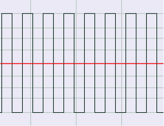
Let’s assume that the microphone or sound level meter is measuring sound amplitude. The sound pressure level of greatest magnitude over a given time period is called the peak amplitude. For a single-frequency sound representable by a sine wave, this would be the level at the peak of the sine wave. The sound represented by Figure 4.3 would obviously be perceived as louder than the same-frequency sound represented by Figure 4.4. However, how would the loudness of a sine-wave-shaped sound compare to the loudness of a square-wave-shaped sound with the same peak amplitude (Figure 4.3 vs. Figure 4.5)? The square wave would actually sound louder. This is because the square wave is at its peak level more of the time as compared to the sine wave. To account for this difference in perceived loudness, RMS amplitude (root-mean-square amplitude) can be used as an alternative to peak amplitude, providing a better match for the way we perceive the loudness of the sound.


Rather than being an instantaneous peak level, RMS amplitude is similar to a standard deviation, a kind of average of the deviation from 0 over time. RMS amplitude is defined as follows:
[equation caption=”Equation 4.9 Equation for RMS amplitude, $$V_{RMS}$$”]
$$!V_{RMS}=\sqrt{\frac{\sum _{i=1}^{n}\left ( S_{i} \right )^{2}}{n}}$$
where n is the number of samples taken and $$S_{i}$$ is the $$i^{th}$$ sample.
[/equation]
[aside]In some sources, the term RMS power is used interchangeably with RMS amplitude or RMS voltage. This isn’t very good usage. To be consistent with the definition of power, RMS power ought to mean “RMS voltage multiplied by RMS current.” Nevertheless, you sometimes see term RMS power used as a synonym of RMS amplitude as defined in Equation 4.9.[/aside]
Notice that squaring each sample makes all the values in the summation positive. If this were not the case, the summation would be 0 (assuming an equal number of positive and negative crests) since the sine wave is perfectly symmetrical.
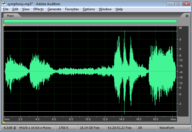
The definition in Equation 4.9 could be applied using whatever units are appropriate for the context. If the samples are being measured as voltages, then RMS amplitude is also called RMS voltage. The samples could also be quantized as values in the range determined by the bit depth, or the samples could also be measured in dimensionless decibels, as shown for Adobe Audition in Figure 4.6.
For a pure sine wave, there is a simple relationship between RMS amplitude and peak amplitude.
[equation caption=”Equation 4.10 Relationship between $$V_{rms}$$ and $$V_{peak}$$ for pure sine waves”]
for pure sine waves
$$!V_{RMS}=\frac{V_{peak}}{\sqrt{2}}=0.707\ast V_{peak}$$
and
$$!V_{peak}=1.414\ast V_{RMS}$$
[/equation]
Of course most of the sounds we hear are not simple waveforms like those shown; natural and musical sounds contain many frequency components that vary over time. In any case, the RMS amplitude is a better model for our perception of the loudness of complex sounds than is peak amplitude.
Sound processing programs often give amplitude statistics as either peak or RMS amplitude or both. Notice that RMS amplitude has to be defined over a particular window of samples, labeled as Window Width in Figure 4.6. This is because the sound wave changes over time. In the figure, the window width is 1000 ms.

You need to be careful will some usages of the term “peak amplitude.” For example, VU meters, which measure signal levels in audio equipment, use the word “peak” in their displays, where RMS amplitude would be more accurate. Knowing this is important when you’re setting levels for a live performance, as the actual peak amplitude is higher than RMS. Transients like sudden percussive noises should be kept well below what is marked as “peak” on a VU meter. If you allow the level to go too high, the signal will be clipped.
4.1.6 Sound Perception
4.1.6.1 Frequency Perception
In Chapter 3, we discussed the non-linear nature of pitch perception when we looked at octaves as defined in traditional Western music. The A above middle C (call it A4) on a piano keyboard sounds very much like the note that is 12 semitones above it, A5, except that A5 has a higher pitch. A5 is one octave higher than A4. A6 sounds like A5 and A4, but it’s an octave higher than A5. The progression between octaves is not linear with respect to frequency. A2’s frequency is twice the frequency of A1. A3’s frequency is twice the frequency of A2, and so forth. A simple way to think of this is that as the frequencies increase by multiplication, the perception of the pitch change increases by addition. In any case, the relationship is non-linear, as you can clearly see if you plot frequencies against octaves, as shown in Figure 4.7.
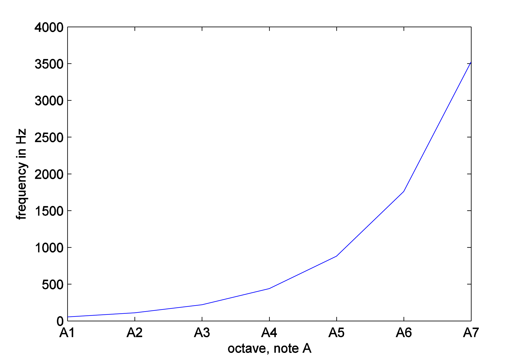
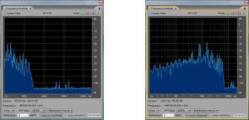
The fact that this is a non-linear relationship implies that the higher up you go in frequencies, the bigger the difference in frequency between neighboring octaves. The difference between A2 and A1 is 110 – 55 = 55 Hz while the difference between A7 and A6 is 3520 – 1760 = 1760 Hz. Because of the non-linearity of our perception, frequency response graphs often show the frequency axis on a logarithmic scale, or you’re given a choice between a linear and a logarithmic scale, as shown in Figure 4.8. Notice that you can select or deselect “linear” in the upper left hand corner. In the figure on the right, the distance between 10 and 100 Hz on the horizontal axis is the same as the distance between 100 and 1000, which is the same as 1000 and 10000. This is more in keeping with how our perception of the pitch changes as the frequencies get higher. You should always pay attention to the scale of the frequency axis in graphs such as this.
The range of frequencies within human hearing is, at best, 20 Hz to 20,000 Hz. The range varies with individuals and diminishes with age, especially for high frequencies. Our hearing is less sensitive to low frequencies than to high; that is, low frequencies have to be more intense for us to hear them than high frequencies.
Frequency resolution (also called frequency discrimination) is our ability to distinguish between two close frequencies. Frequency resolution varies by frequency, loudness, the duration of the sound, the suddenness of the frequency change, and the acuity and training of the listener’s ears. The smallest frequency change that can be noticed as a pitch change is referred to as a just-noticeable-difference (jnd). At low frequencies, it’s possible to notice a difference between frequencies that are separated by just a few Hertz. Within the 1000 Hz to 4000 Hz range, it’s possible for a person to hear a jnd of as little as 1/12 of a semitone. (But 1/12 a semitone step from 1000 Hz is about 88 Hz, while 1/12 a semitone step from 4000 Hz is about 353 Hz.) At low frequencies, tones that are separated by just a few Hertz can be distinguished as separate pitches, while at high frequencies, two tones must be separated by hundreds of Hertz before a difference is noticed.
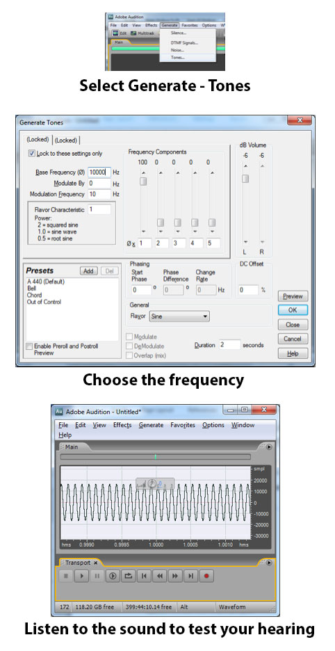
You can test your own frequency range and discrimination with a sound processing program like Audacity or Audition, generating and listening to pure tones, as shown in Figure 4.9 Be aware, however, that the monitors or headphones you use have an impact on your ability to hear the frequencies.
4.1.6.2 Critical Bands
One part of the ear’s anatomy that is helpful to consider more closely is the area in the inner ear called the basilar membrane. It is here that sound vibrations are detected, separated by frequencies, and transformed from mechanical energy to electrical impulses sent to the brain. The basilar membrane is lined with rows of hair cells and thousands of tiny hairs emanating from them. The hairs move when stimulated by vibrations, sending signals to their base cells and the attached nerve fibers, which pass electrical impulses to the brain. In his pioneering work on frequency perception, Harvey Fletcher discovered that different parts of the basilar membrane resonate more strongly to different frequencies. Thus, the membrane can be divided into frequency bands, commonly called critical bands. Each critical band of hair cells is sensitive to vibrations within a certain band of frequencies. Continued research on critical bands has shown that they play an important role in many aspects of human hearing, affecting our perception of loudness, frequency, timbre, and dissonance vs. consonance. Experiments with critical bands have also led to an understanding of frequency masking, a phenomenon that can be put to good use in audio compression.
Critical bands can be measured by the band of frequencies that they cover. Fletcher discovered the existence of critical bands in his pioneering work on the cochlear response. Critical bands are the source of our ability to distinguish one frequency from another. When a complex sound arrives at the basilar membrane, each critical band acts as a kind of bandpass filter, responding only to vibrations within its frequency spectrum. In this way, the sound is divided into frequency components. If two frequencies are received within the same band, the louder frequency can overpower the quieter one. This is the phenomenon of masking, first observed in Fletcher’s original experiments.
[aside]A bandpass filter allows only the frequencies in a defined band to pass through, filtering out all other frequencies. Bandpass filters are studied in Chapter 7.[/aside]
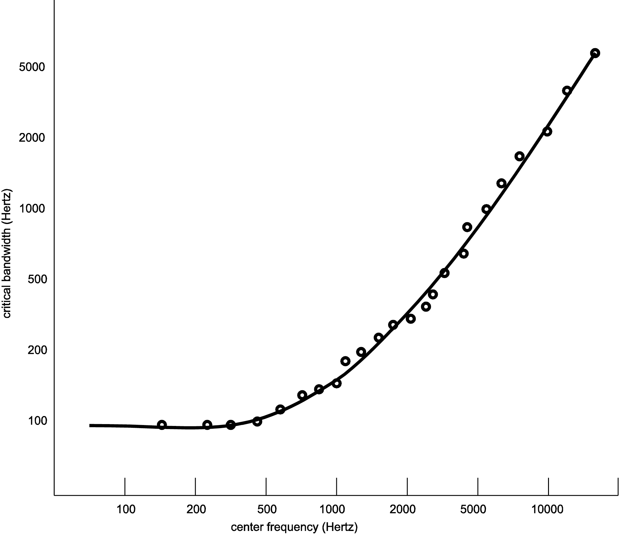
Critical bands within the ear are not fixed areas but instead are created during the experience of sound. Any audible sound can create a critical band centered on it. However, experimental analyses of critical bands have arrived at approximations that are useful guidelines in designing audio processing tools. Table 4.4 is one model taken after Fletcher, Zwicker, and Barkhausen’s independent experiments, as cited in (Tobias, 1970). Here, the basilar membrane is divided into 25 overlapping bands, each with a center frequency and with variable bandwidths across the audible spectrum. The width of each band is given in Hertz, semitones, and octaves. (The widths in semitones and octaves were derived from the widths in Hertz, as explained in Section 4.3.1.) The center frequencies are graphed against the critical bands in Hertz in Figure 4.10.
You can see from the table and figure that, measured in Hertz, the critical bands are wider for higher frequencies than for lower. This implies that there is better frequency resolution at lower frequencies because a narrower band results in less masking of frequencies in a local area.
The table shows that critical bands are generally in the range of two to four semitones wide, mostly less than four. This observation is significant as it relates to our experience of consonance vs. dissonance. Recall from Chapter 3 that a major third consists of four semitones. For example, the third from C to E is separated by four semitones (stepping from C to C#, C# to D, D to D #, and D# to E.) Thus, the notes that are played simultaneously in a third generally occupy separate critical bands. This helps to explain why thirds are generally considered consonant – each of the notes having its own critical band. Seconds, which exist in the same critical band, are considered dissonant. At very low and very high frequencies, thirds begin to lose their consonance to most listeners. This is consistent with the fact that the critical bands at the low frequencies (100-200 and 200-300 Hz) and high frequencies (over 12000 Hz) span more than a third, so that at these frequencies, a third lies within a single critical band.
[table caption=”Table 4.4 An estimate of critical bands using the Bark scale” width=”80%”]
Critical Band,Center Frequency in Hertz,Range of Frequencies in Hertz,Bandwidth in Hertz,Bandwidth in Semitones Relative to Start*,Bandwidth in Octaves Relative to Start*
1,50,1-100,100,,-
2,150,100-200,100,12,1
3,250,200-300,100,7,0.59
4,350,300–400,100,5,0.42
5,450,400–510,110,4,0.31
6,570,510–630,120,4,0.3
7,700,630–770,140,3,0.29
8,840,770–920,150,3,0.26
9,1000,920–1080,160,3,0.23
10,1170,1080–1270,190,3,0.23
11,1370,1270–1480,210,3,0.22
12,1600,1480–1720,240,3,0.22
13,1850,1720–2000,280,3,0.22
14,2150,2000–2320,320,3,0.21
15,2500,2320–2700,380,3,0.22
16,2900,2700–3150,450,3,0.22
17,3400,3150–3700,550,3,0.23
18,4000,3700–4400,700,3,0.25
19,4800,4400–5300,900,3,0.27
20,5800,5300–6400,1100,3,0.27
21,7000,6400–7700,1300,3,0.27
22,8500,7700–9500,1800,4,0.3
23,10500,9500–12000,2500,4,0.34
24,13500,12000–15500,3500,4,0.37
25,18775,15500–22050,6550,6,0.5
*See Section 4.3.2 for an explanation of how the last two columns of this table were derived.[attr colspan=”6″]
[/table]
4.1.6.3 Amplitude Perception
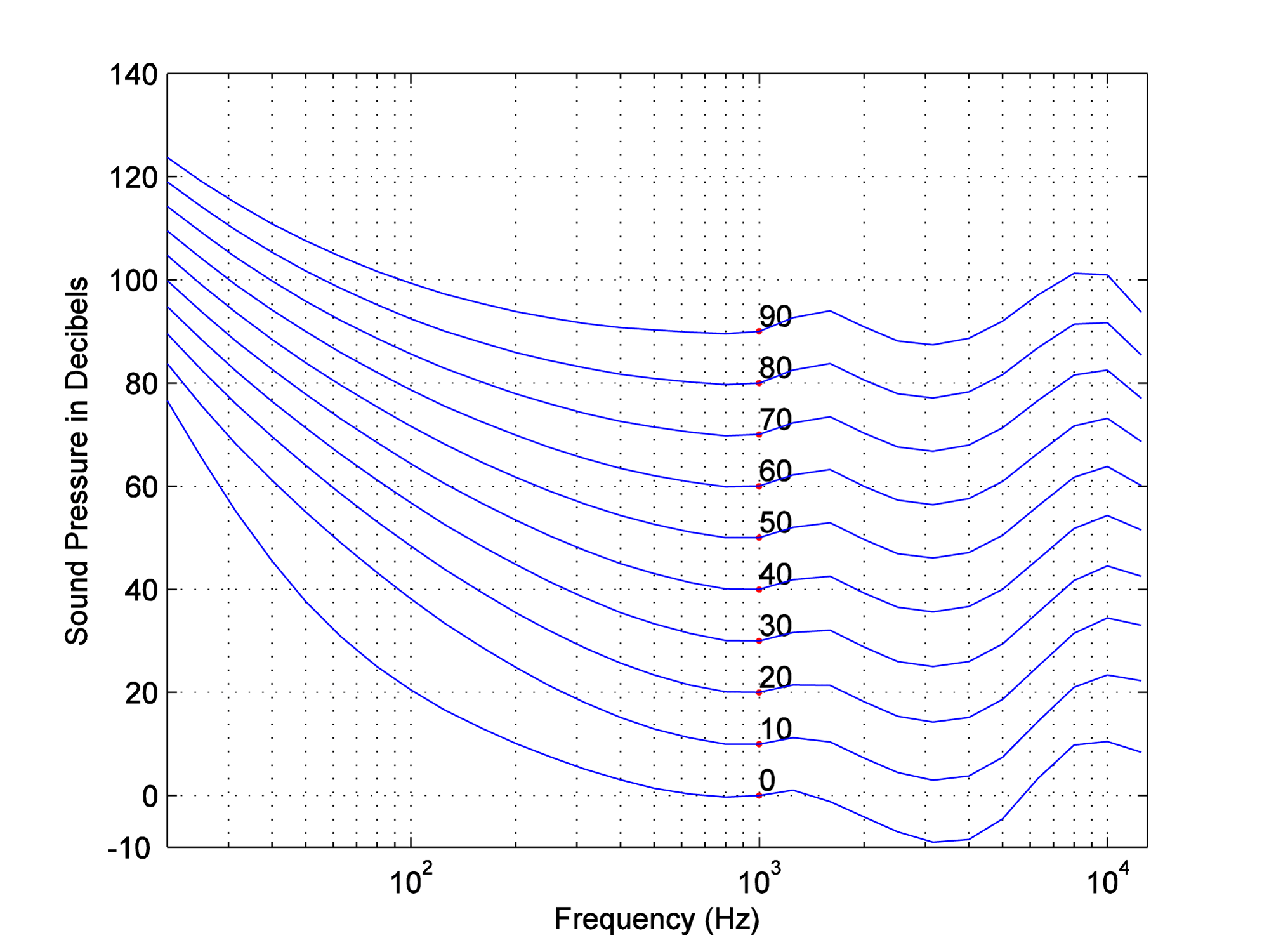
In the early 1930s at Bell Laboratories, groundbreaking experiments by Fletcher and Munson clarified the extent to which our perception of loudness varies with frequency (Fletcher and Munson 1933). Their results, refined by later researchers (Robinson and Dadson, 1956) and adopted as International Standard ISO 226, are illustrated in a graph of equal-loudness contours shown in Figure 4.11. In general, the graph shows how much you have to “turn up” or “turn down” a single frequency tone to make it sound equally loud to a 1000 Hz tone. Each curve on the graph represents an n-phon contour. One phon is defined as a 1000 Hz sound wave at a loudness of 1 dBSPL. An n-phon contour is created as follows:
- Frequency is on the horizontal axis and loudness in decibels is on the vertical axis
- n curves are drawn.
- Each curve, from 1 to n, represents the intensity levels necessary in order to make each frequency, across the audible spectrum, sound equal in loudness to a 1000 Hz wave at n dBSPL.
Let’s consider, for example, the 10-phon contour. This contour was creating by playing a 1000 Hz pure tone at a loudness level of 10 dBSPL, and then asking groups of listeners to say when they thought pure tones at other frequencies matched the loudness of the 1000 Hz tone. Notice that low-frequency tones had to be increased by 60 or 75 dB to sound equally loud. Some of the higher-frequency tones – in the vicinity of 3000 Hz – actually had to be turned down in volume to sound equally loud to the 10 dBSPL 1000 Hz tone. Also notice that the louder the 1000 Hz tone is, the less lower-frequency tones have to be turned up to sound equal in loudness. For example, the 90-phon contour goes up only about 30 dB to make the lowest frequencies sound equal in loudness to 1000 Hz at 90 dBSPL, whereas the 10-phon contour has to be turned up about 75 dB.
With the information captured in the equal loudness contours, devices that measure the loudness of sounds – for example, SPL meters (sound pressure level meters) – can be designed so that they compensate for the fact that low frequency sounds seem less loud than high frequency sounds at the same amplitude. This compensation is called “weighting.” Figure 4.12 graphs three weighting functions – A, B, and C. The A, B, and C-weighting functions are approximately inversions of the 40-phon, 70-phon, and 100-phon loudness contours, respectively. This implies that applying A-weighting in an SPL meter causes the meter to measure loudness in a way that matches our differences in loudness perception at 40-phons.
To understand how this works, think of the graphs of the weighting as frequency filters – also called frequency response graphs. When a weighting function is applied by an SPL meter, the meter uses a filter to reduce the influence of frequencies to which our ears are less sensitive, and conversely to increase the weight of frequencies that our ears are sensitive to. The fact that the A-weighting graph is lower on the left side than on the right means that an A-weighted SPL meter reduces the influence of low-frequency sounds as it takes its overall loudness measurement. On the other hand, it boosts the amplitude of frequencies around 3000 Hz, as seen by the bump above 0 dB around 3000 Hz. It doesn’t matter that the SPL meter meddles with frequency components as it measures loudness. After all, it isn’t measuring frequencies. It’s measuring how loud the sounds seem to our ears. The use of weighted SPL meters is discussed further in Section 4.2.2.2.
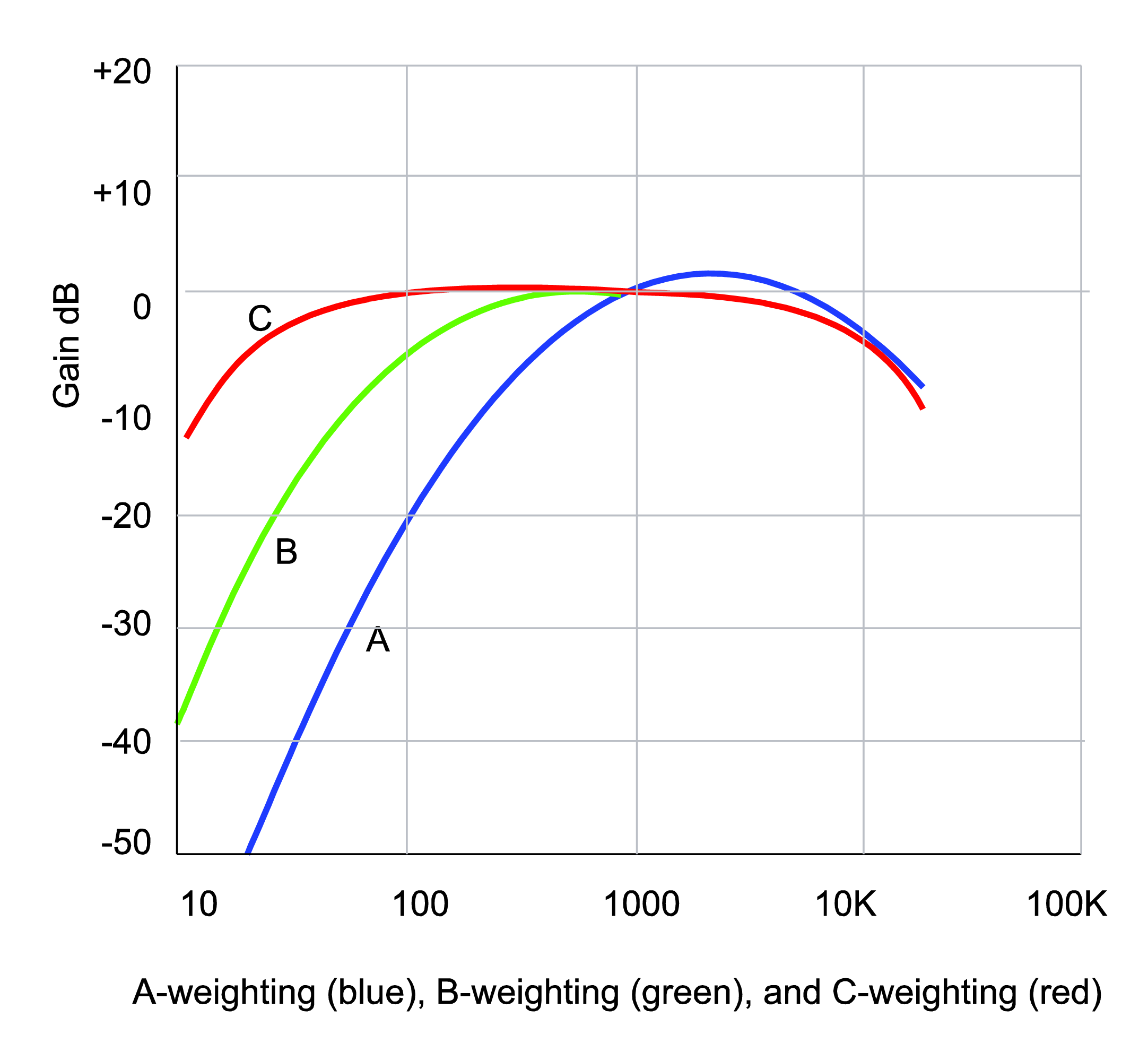
(Figure derived from a program by Jeff Tacket, posted at the MATLAB Central File Exchange)
4.1.7 The Interaction of Sound with its Environment
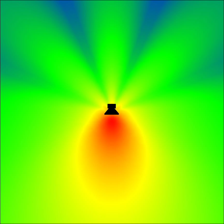
Sometimes it’s convenient to simplify our understanding of sound by considering how it behaves when there is nothing in the environment to impede it. An environment with no physical influences to absorb, reflect, diffract, refract, reverberate, resonate, or diffuse sound is called a free field. A free field is an idealization of real world conditions that facilitates our analysis of how sound behaves. Sound in a free field can be pictured as radiating out from a point source, diminishing in intensity as it gets farther from the source. A free field is partially illustrated in Figure 4.18. In this figure, sound is radiating out from a loudspeaker, with the colors indicating highest to lowest intensity sound in the order red, orange, yellow, green, and blue. The area in front of the loudspeaker might be considered a free field. However, because the loudspeaker partially blocks the sound from going behind itself, the sound is lower in amplitude there. You can see that there is some sound behind the loudspeaker, resulting from reflection and diffraction.
4.1.7.1 Absorption, Reflection, Refraction, and Diffraction
In the real world, there are any number of things that can get in the way of sound, changing its direction, amplitude, and frequency components. In enclosed spaces, absorption plays an important role. Sound absorption is the conversion of sound’s energy into heat, thereby diminishing the intensity of the sound. The diminishing of sound intensity is called attenuation. A general mathematical formulation for the way sound attenuates as it moves through the air is captured in the inverse square law, which shows that sound decreases in intensity in proportion to the square of the distance from the source. (See Section 4.2.1.6.) The attenuation of sound in the air is due to the air molecules themselves absorbing and converting some of the energy to heat. The amount of attenuation depends in part on the air temperature and relative humidity. Thick, porous materials can absorb and attenuate the sound even further, and they’re often used in architectural treatments to modify and control the acoustics of a room. Even hard, solid surfaces absorb some of the sound energy, although most of it is reflected back. The material of walls and ceilings, the number and material of seats, the number of persons in an audience, and all solid objects have to be taken into consideration acoustically in sound setups for live performance spaces.
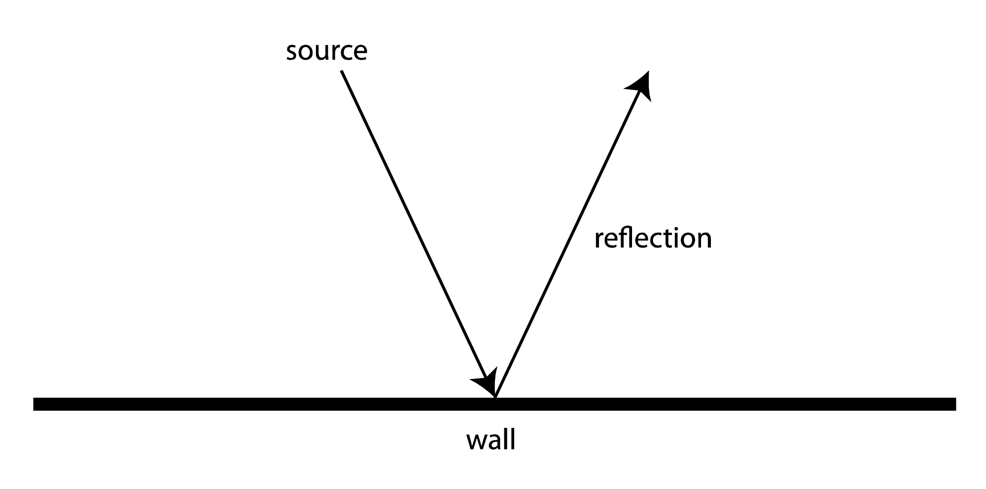
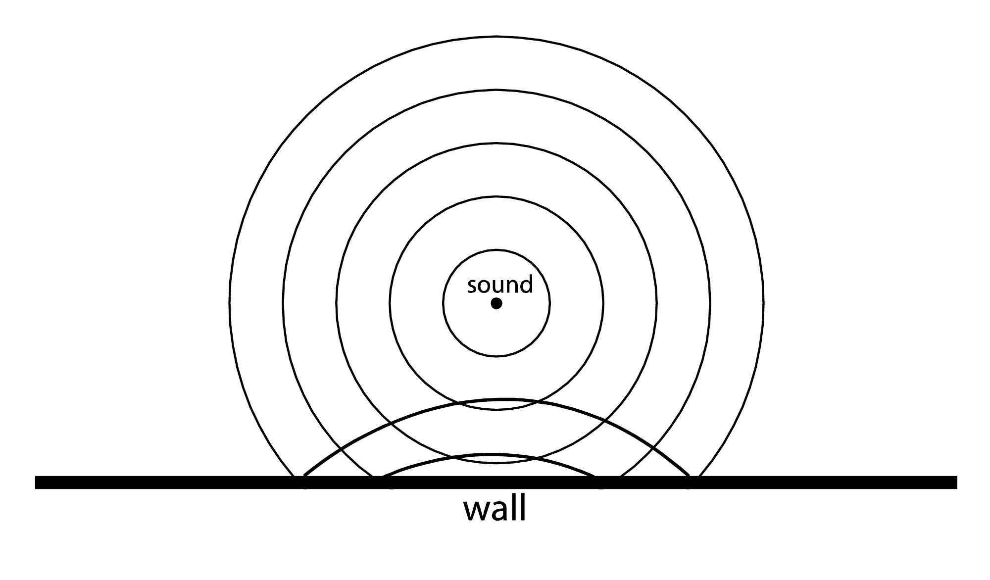
Sound that is not absorbed by objects is instead reflected from, diffracted around, or refracted into the object. Hard surfaces reflect sound more than soft ones, which are more absorbent. The law of reflection states that the angle of incidence of a wave is equal to the angle of reflection. This means that if a wave were to propagate in a straight line from its source, it reflects in the way pictured in Figure 4.15. In reality, however, sound radiates out spherically from its source. Thus, a wavefront of sound approaches objects and surfaces from various angles. Imagine a cross-section of the moving wavefront approaching a straight wall, as seen from above. Its reflection would be as pictured in Figure 4.15, like a mirror reflection.
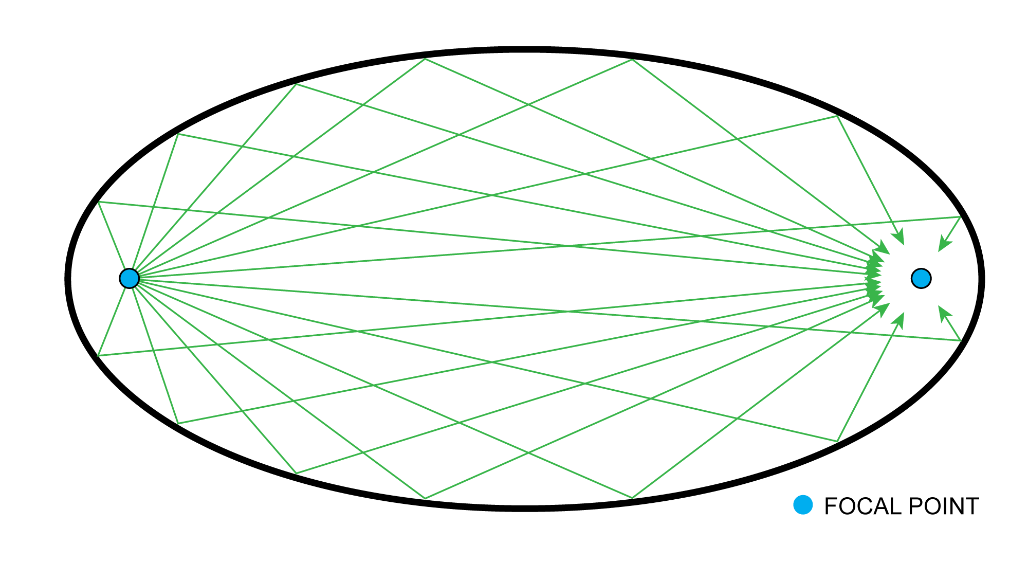
In a special case, if the wavefront were to approach a concave curved solid surface, it would be reflected back to converge at one point in the room, the location of that point depending on the angle of the curve. This is how whispering rooms are constructed, such that two people whispering in the room can hear each other perfectly if they’re positioned at the sound’s focal points, even though the focal points may be at the far opposite ends of the room. A person positioned elsewhere in the room cannot hear their whispers at all. A common shape found with whispering rooms is an ellipse, as seen in Figure 4.16. The shape and curve of these walls cause any and all sound emanating from one focal point to reflect directly to the other.
[aside]
Diffraction also has a lot to do with microphone and loudspeaker directivity. Consider how microphones often have different polar patterns at different frequencies. Even with a directional mic, you’ll often see lower frequencies behave more omnidirectionally, and sometimes an omnidirectional mic may be more directional at high frequencies. That’s largely because of the size of the wavelength compared to size of the microphone diaphragm. It’s hard for high frequencies to diffract around a larger object, so for a mic to have a truly omnidirectional pattern, the diaphragm has to be very small.
[/aside]
Diffraction is the bending of a sound wave as it moves past an obstacle or through a narrow opening. The phenomenon of diffraction allows us to hear sounds from sources that are not in direct line-of-sight, such as a person standing around a corner or on the other side of a partially obstructing object. The amount of diffraction is dependent on the relationship between the size of the obstacle and the size of the sound’s wavelength. Low frequency sounds (i.e., long-wavelength sounds) are diffracted more than high frequencies (i.e., short wavelengths) around the same obstacle. In other words, low frequency sounds are better able to travel around obstacles. In fact, if the wavelength of a sound is significantly larger than an obstacle that the sound encounters, the sound wave continues as if the obstacle isn’t even there. For example, your stereo speaker drivers are probably protected behind a plastic or metal grill, yet the sound passes through it intact and without noticeable coloration. The obstacle presented by the wire mesh of the grill (perhaps a millimeter or two in diameter) is even smaller than the smallest wavelength we can hear (about 2 centimeters for 20 kHz, 10 to 20 times larger than the wire), so the sound diffracts easily around it.
Refraction is the bending of a sound wave as it moves through different media. Typically we think of refraction with light waves, as when we look at something through glass or that is underwater. In acoustics, the refraction of sound waves tends to be more gradual, as the properties of the air change subtly over longer distances. This causes a bending in sound waves over a long distance, primarily due to temperature, humidity, and in some cases wind gradients over distance and altitude. This bending can result in noticeable differences in sound levels, either as a boost or an attenuation, also referred to as a shadow zone.
4.1.7.2 Reverberation, Echo, Diffusion, and Resonance
Reverberation is the result of sound waves reflecting off of many objects or surfaces in the environment. Imagine an indoor room in which you make a sudden burst of sound. Some of that sound is transmitted through or absorbed by the walls or objects, and the rest is reflected back, bouncing off the walls, ceilings, and other surfaces in the room. The sound wave that travels straight from the sound source to your ears is called the direct signal. The first few instances of reflected sound are called primary or early reflections. Early reflections arrive at your ears about 60 ms or sooner after the direct sound, and play a large part in imparting a sense of space and room size to the human ear. Early reflections may be followed by a handful of secondary and higher-order reflections. At this point, the sound waves have had plenty of opportunity to bounce off of multiple surfaces, multiple times. As a result, the reflections that are arriving now are more numerous, closer together in time, and quieter. Much of the initial energy initial energy of the reflections has been absorbed by surfaces or expended in the distance traveled through the air. This dense collection of reflections is reverberation, illustrated in Figure 4.17. Assuming that the sound source is only momentary, the generated sound eventually decays as the waves lose energy, the reverberation becoming less and less loud until the sound is no longer discernable. Typically, reverberation time is defined as the time it takes for the sound to decay in level by 60 dB from its direct signal.

Single, strong reflections that reach the ear a significant amount of time – about 100 ms – after the direct signal can be perceived as an echo – essentially a separate recurrence of the original sound. Even reflections as little as 50 ms apart can cause an audible echo, depending on the type of sound and room acoustics. While echo is often employed artistically in music recordings, echoes tend to be detrimental and distracting in a live setting and are usually avoided or require remediation in performance and listening spaces.
Diffusion is another property that interacts with reflections and reverberation. Diffusion relates to the ability to distribute sound energy more evenly in a listening space. While a flat, even surface reflects sounds strongly in a predictable direction, uneven surfaces or convex curved surfaces diffuse sound more randomly and evenly. Like absorption, diffusion is often used to treat a space acoustically to help break up harsh reflections that interfere with the natural sound. Unlike absorption, however, which attempts to eliminate the unwanted sound waves by reducing the sound energy, diffusion attempts to redirect the sound waves in a more natural manner. A room with lots of absorption has less overall reverberation, while diffusion maintains the sound’s intensity and helps turn harsh reflections into more pleasant reverberation. Usually a combination of absorption and diffusion is employed to achieve the optimal result. There are many unique types of diffusing surfaces and panels that are manufactured based on mathematical algorithms to provide the most random, diffuse reflections possible
Putting these concepts together, we can say that the amount of time it takes for a particular sound to decay depends on the size and shape of the room, its diffusive properties, and the absorptive properties of the walls, ceilings, and objects in the room. In short, all the aforementioned properties determine how sound reverberates in a space, giving the listener a “sense of place.”
Reverberation in an auditorium can enhance the listener’s experience, particularly in the case of a music hall where it gives the individual sounds a richer quality and helps them blend together. Excessive reverberation, however, can reduce intelligibility and make it difficult to understand speech. In Chapter 7, you’ll see how artificial reverberation is applied in audio processing.
A final important acoustical property to be considered is resonance. In Chapter 2, we defined resonance as an object’s tendency to vibrate or oscillate at a certain frequency that is basic to its nature. Like a musical instrument, a room has a set of resonant frequencies, called its room modes. Room modes result in locations in a room where certain frequencies are boosted or attenuated, making it difficult to give all listeners the same audio experience. We’ll talk more about how to deal with room modes in Section 4.2.2.5.