2.1.1 Sound Waves, Sine Waves, and Harmonic Motion
Working with digital sound begins with an understanding of sound as a physical phenomenon. The sounds we hear are the result of vibrations of objects – for example, the human vocal chords, or the metal strings and wooden body of a guitar. In general, without the influence of a specific sound vibration, air molecules move around randomly. A vibrating object pushes against the randomly-moving air molecules in the vicinity of the vibrating object, causing them first to crowd together and then to move apart. The alternate crowding together and moving apart of these molecules in turn affects the surrounding air pressure. The air pressure around the vibrating object rises and falls in a regular pattern, and this fluctuation of air pressure, propagated outward, is what we hear as sound.
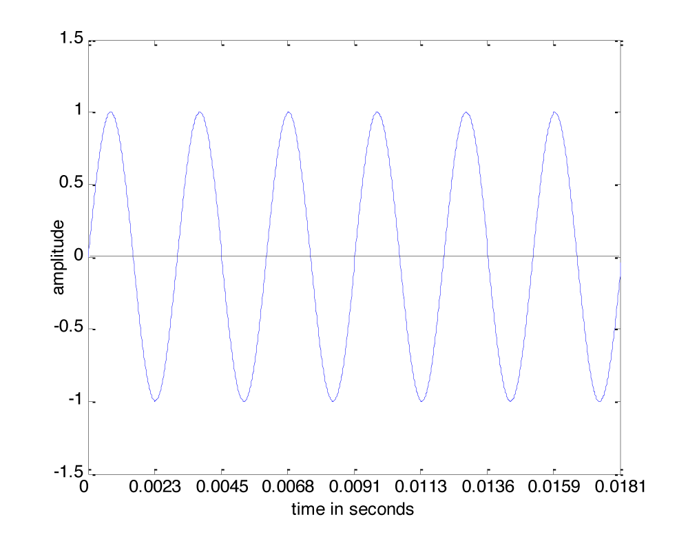
Sound is often referred to as a wave, but we need to be careful with the commonly-used term “sound wave,” as it can lead to a misconception about the nature of sound as a physical phenomenon. On the one hand, there’s the physical wave of energy passed through a medium as sound travels from its source to a listener. (We’ll assume for simplicity that the sound is traveling through air, although it can travel through other media.) Related to this is the graphical view of sound, a plot of air pressure amplitude at a particular position in space as it changes over time. For single-frequency sounds, this graph takes the shape of a “wave,” as shown in Figure 2.1. More precisely, a single-frequency sound can be expressed as a sine function and graphed as a sine wave (as we’ll describe in more detail later). Let’s see how these two things are related.
[wpfilebase tag=file id=105 tpl=supplement /]
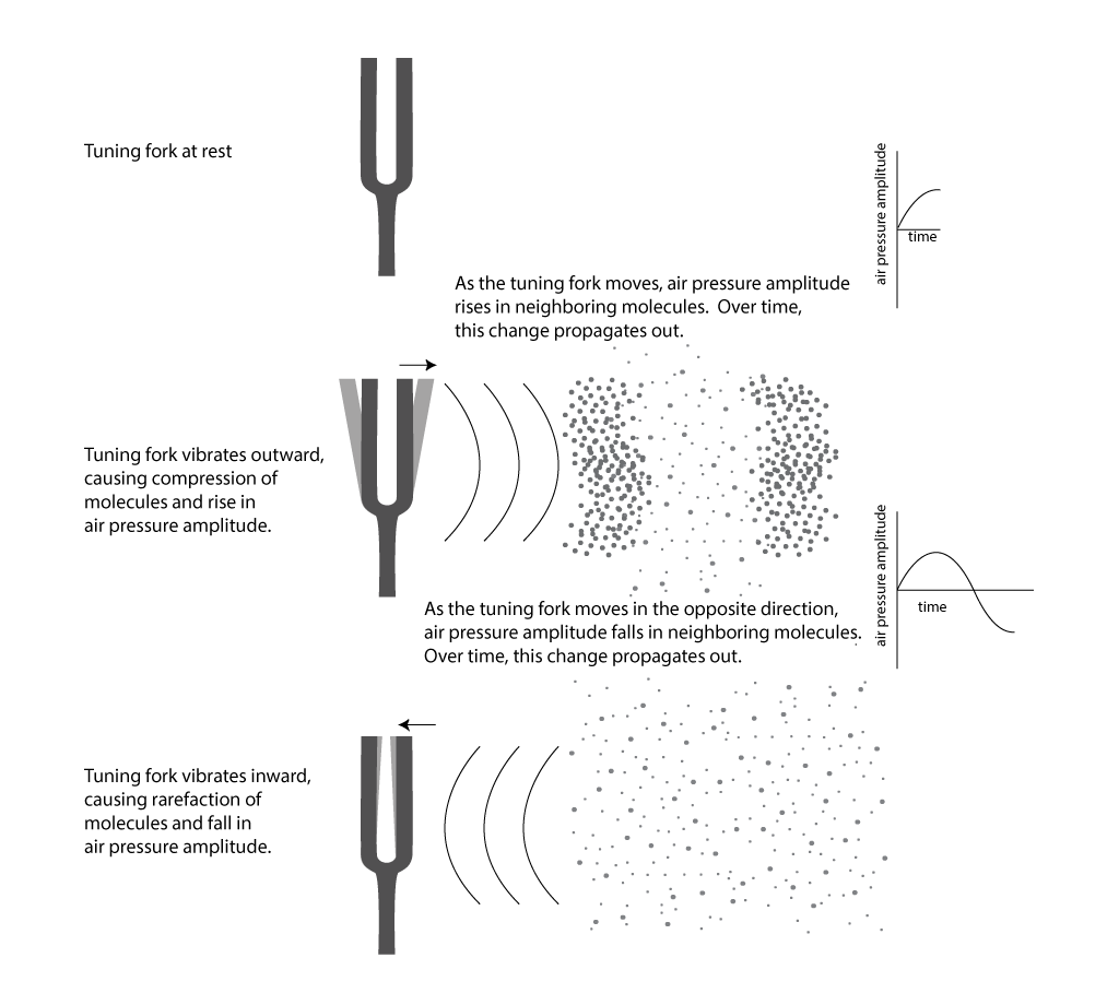
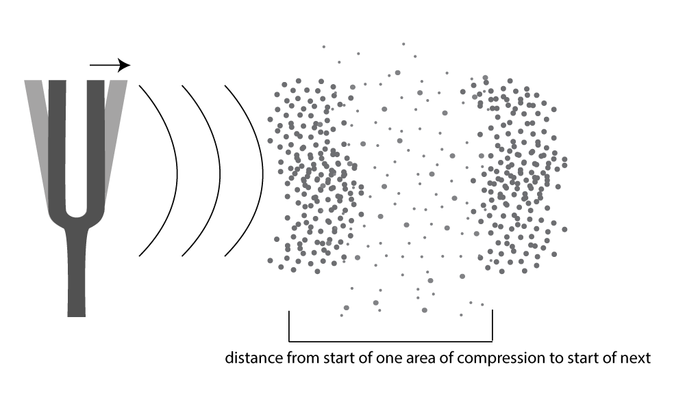
First, consider a very simple vibrating object – a tuning fork. When the tuning fork is struck, it begins to move back and forth. As the prong of the tuning fork vibrates outward (in Figure 2.2), it pushes the air molecules right next to it, which results in a rise in air pressure corresponding to a local increase in air density. This is called compression. Now, consider what happens when the prong vibrates inward. The air molecules have more room to spread out again, so the air pressure beside the tuning fork falls. The spreading out of the molecules is called decompression or rarefaction. A wave of rising and falling air pressure is transmitted to the listener’s ear. This is the physical phenomenon of sound, the actual sound wave.
Assume that a tuning fork creates a single-frequency wave. Such a sound wave can be graphed as a sine wave, as illustrated in Figure 2.1. An incorrect understanding of this graph would be to picture air molecules going up and down as they travel across space from the place in which the sound originates to the place in which it is heard. This would be as if a particular molecule starts out where the sound originates and ends up in the listener’s ear. This is not what is being pictured in a graph of a sound wave. It is the energy, not the air molecules themselves, that is being transmitted from the source of a sound to the listener’s ear. If the wave in Figure 2.1 is intended to depict a single-frequency sound wave, then the graph has time on the x-axis (the horizontal axis) and air pressure amplitude on the y-axis. As described above, the air pressure rises and falls. For a single-frequency sound wave, the rate at which it does this is regular and continuous, taking the shape of a sine wave.
Thus, the graph of a sound wave is a simple sine wave only if the sound has only one frequency component in it – that is, just one pitch. Most sounds are composed of multiple frequency components – multiple pitches. A sound with multiple frequency components also can be represented as a graph which plots amplitude over time; it’s just a graph with a more complicated shape. For simplicity, we sometimes use the term “sound wave” rather than “graph of a sound wave” for such graphs, assuming that you understand the difference between the physical phenomenon and the graph representing it.
The regular pattern of compression and rarefaction described above is an example of harmonic motion, also called harmonic oscillation. Another example of harmonic motion is a spring dangling vertically. If you pull on the bottom of the spring, it will bounce up and down in a regular pattern. Its position – that is, its displacement from its natural resting position – can be graphed over time in the same way that a sound wave’s air pressure amplitude can be graphed over time. The spring’s position increases as the spring stretches downward, and it goes to negative values as it bounces upwards. The speed of the spring’s motion slows down as it reaches its maximum extension, and then it speeds up again as it bounces upwards. This slowing down and speeding up as the spring bounces up and down can be modeled by the curve of a sine wave. In the ideal model, with no friction, the bouncing would go on forever. In reality, however, friction causes a damping effect such that the spring eventually comes to rest. We’ll discuss damping more in a later chapter.
Now consider how sound travels from one location to another. The first molecules bump into the molecules beside them, and they bump into the next ones, and so forth as time goes on. It’s something like a chain reaction of cars bumping into one another in a pile-up wreck. They don’t all hit each other simultaneously. The first hits the second, the second hits the third, and so on. In the case of sound waves, this passing along of the change in air pressure is called sound wave propagation. The movement of the air molecules is different from the chain reaction pile up of cars, however, in that the molecules vibrate back and forth. When the molecules vibrate in the direction opposite of their original direction, the drop in air pressure amplitude is propagated through space in the same way that the increase was propagated.
Be careful not to confuse the speed at which a sound wave propagates and the rate at which the air pressure amplitude changes from highest to lowest. The speed at which the sound is transmitted from the source of the sound to the listener of the sound is the speed of sound. The rate at which the air pressure changes at a given point in space – i.e., vibrates back and forth – is the frequency of the sound wave. You may understand this better through the following analogy. Imagine that you’re watching someone turn a flashlight on and off, repeatedly, at a certain fixed rate in order to communicate a sequence of numbers to you in binary code. The image of this person is transmitted to your eyes at the speed of light, analogous to the speed of sound. The rate at which the person is turning the flashlight on and off is the frequency of the communication, analogous to the frequency of a sound wave.
The above description of a sound wave implies that there must be a medium through which the changing pressure propagates. We’ve described sound traveling through air, but sound also can travel through liquids and solids. The speed at which the change in pressure propagates is the speed of sound. The speed of sound is different depending upon the medium in which sound is transmitted. It also varies by temperature and density. The speed of sound in air is approximately 1130 ft/s (or 344 m/s). Table 2.1 shows the approximate speed in other media.
[table caption=”Table 2.1 The Speed of sound in various media” colalign=”center|center|center” width=”80%”]
Medium,Speed of sound in m/s, Speed of sound in ft/s
“air (20° C, which is 68° F)”,344,”1,130″
“water (just above 0° C, which is 32° F)”,”1,410″,”4,626″
steel,”5,100″,”16,700″
lead,”1,210″,”3,970″
glass,”approximately 4,000~~(depending on type of glass)”,”approximately 13,200″
[/table]
[aside width=”75px”]
feet = ft
seconds = s
meters = m
[/aside]
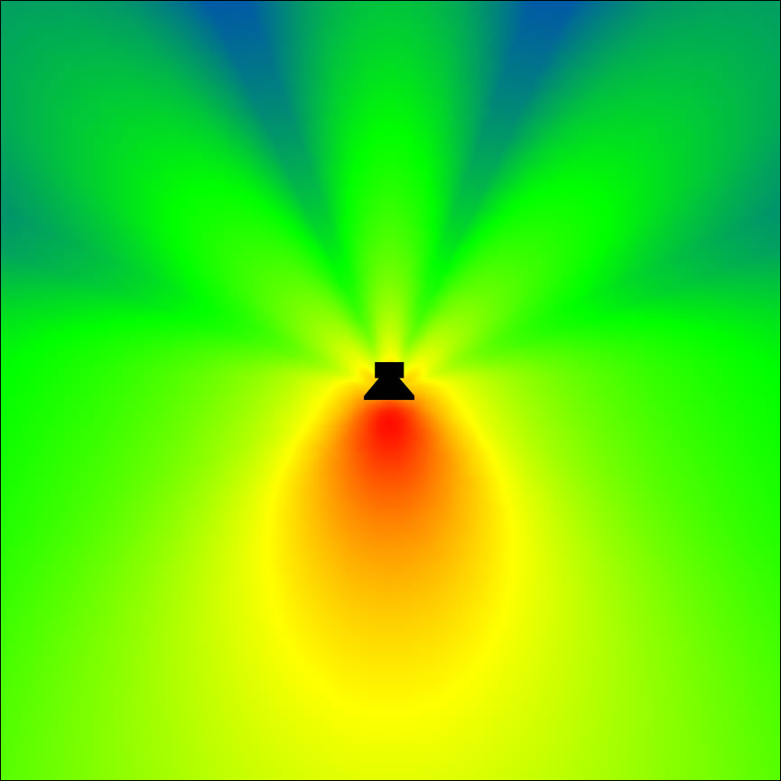
For clarity, we’ve thus far simplified the picture of how sound propagates. Figure 2.2 makes it look as though there’s a single line of sound going straight out from the tuning fork and arriving at the listener’s ear. In fact, sound radiates out from a source at all angles in a sphere. Figure 2.3 shows a top-view image of a real sound radiation pattern, generated by software that uses sound dispersion data, measured from an actual loudspeaker, to predict how sound will propagate in a given three-dimensional space. In this case, we’re looking at the horizontal dispersion of the loudspeaker. Colors are used to indicate the amplitude of sound, going highest to lowest from red to yellow to green to blue. The figure shows that the amplitude of the sound is highest in front of the loudspeaker and lowest behind it. The simplification in Figure 2.2 suffices to give you a basic concept of sound as it emanates from a source and arrives at your ear. Later, when we begin to talk about acoustics, we’ll consider a more complete picture of sound waves.
Sound waves are passed through the ear canal to the eardrum, causing vibrations which pass to little hairs in the inner ear. These hairs are connected to the auditory nerve, which sends the signal onto the brain. The rate of a sound vibration – its frequency – is perceived as its pitch by the brain. The graph of a sound wave represents the changes in air pressure over time resulting from a vibrating source. To understand this better, let’s look more closely at the concept of frequency and other properties of sine waves.
2.1.2 Properties of Sine Waves
We assume that you have some familiarity with sine waves from trigonometry, but even if you don’t, you should be able to understand some basic concepts of this explanation.
A sine wave is a graph of a sine function . In the graph, the x-axis is the horizontal axis, and the y-axis is the vertical axis. A graph or phenomenon that takes the shape of a sine wave – oscillating up and down in a regular, continuous manner – is called a sinusoid.
In order to have the proper terminology to discuss sound waves and the corresponding sine functions, we need to take a little side trip into mathematics. We’ll first give the sine function as it applies to sound, and then we’ll explain the related terminology.
[equation caption=”Equation 2.1″]A single-frequency sound wave with frequency f , maximum amplitude A, and phase θ is represented by the sine function
$$!y=A\sin \left ( 2\pi fx+\theta \right )$$
where x is time and y is the amplitude of the sound wave at time x.[/equation]
[wpfilebase tag=file id=106 tpl=supplement /]
Single-frequency sound waves are sinusoidal waves. Although pure single-frequency sound waves do not occur naturally, they can be created artificially by means of a computer. Naturally occurring sound waves are combinations of frequency components, as we’ll discuss later in this chapter.
The graph of a sound wave is repeated Figure 2.4 with some of its parts labeled. The amplitude of a wave is its y value at some moment in time given by x. If we’re talking about a pure sine wave, then the wave’s amplitude, A, is the highest y value of the wave. We call this highest value the crest of the wave. The lowest value of the wave is called the trough. When we speak of the amplitude of the sine wave related to sound, we’re referring essentially to the change in air pressure caused by the vibrations that created the sound. This air pressure, which changes over time, can be measured in Newtons/meter2 or, more customarily, in decibels (abbreviated dB), a logarithmic unit explained in detail in Chapter 4. Amplitude is related to perceived loudness. The higher the amplitude of a sound wave, the louder it seems to the human ear.
In order to define frequency, we must first define a cycle. A cycle of a sine wave is a section of the wave from some starting position to the first moment at which it returns to that same position after having gone through its maximum and minimum amplitudes. Usually, we choose the starting position to be at some position where the wave crosses the x-axis, or zero crossing, so the cycle would be from that position to the next zero crossing where the wave starts to repeat, as shown in Figure 2.4.
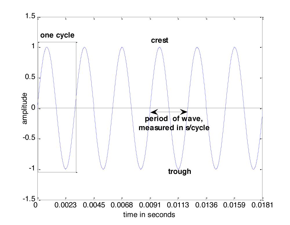
The frequency of a wave, f, is the number of cycles per unit time, customarily the number of cycles per second. A unit that is used in speaking of sound frequency is Hertz, defined as 1 cycle/second, and abbreviated Hz. In Figure 2.4, the time units on the x-axis are seconds. Thus, the frequency of the wave is 6 cycles/0.0181 seconds » 331 Hz. Henceforth, we’ll use the abbreviation s for seconds and ms for milliseconds.
Frequency is related to pitch in human perception. A single-frequency sound is perceived as a single pitch. For example, a sound wave of 440 Hz sounds like the note A on a piano (just above middle C). Humans hear in a frequency range of approximately 20 Hz to 20,000 Hz. The frequency ranges of most musical instruments fall between about 50 Hz and 5000 Hz. The range of frequencies that an individual can hear varies with age and other individual factors.
The period of a wave, T, is the time it takes for the wave to complete one cycle, measured in s/cycle. Frequency and period have an inverse relationship, given below.
[equation caption=”Equation 2.2″]Let the frequency of a sine wave be and f the period of a sine wave be T. Then
$$!f=1/T$$
and
$$!T=1/f$$
[/equation]
The period of the wave in Figure 2.4 is about three milliseconds per cycle. A 440 Hz wave (which has a frequency of 440 cycles/s) has a period of 1 s/440 cycles, which is about 0.00227 s/cycle. There are contexts in which it is more convenient to speak of period only in units of time, and in these contexts the “per cycle” can be omitted as long as units are handled consistently for a particular computation. With this in mind, a 440 Hz wave would simply be said to have a period of 2.27 milliseconds.
[wpfilebase tag=file id=28 tpl=supplement /]
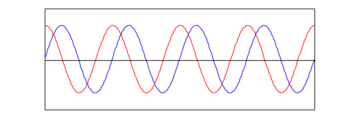
The phase of a wave, θ, is its offset from some specified starting position at x = 0. The sine of 0 is 0, so the blue graph in Figure 2.5 represents a sine function with no phase offset. However, consider a second sine wave with exactly the same frequency and amplitude, but displaced in the positive or negative direction on the x-axis relative to the first, as shown in Figure 2.5. The extent to which two waves have a phase offset relative to each other can be measured in degrees. If one sine wave is offset a full cycle from another, it has a 360 degree offset (denoted 360o); if it is offset a half cycle, is has a 180 o offset; if it is offset a quarter cycle, it has a 90 o offset, and so forth. In Figure 2.5, the red wave has a 90 o offset from the blue. Equivalently, you could say it has a 270 o offset, depending on whether you assume it is offset in the positive or negative x direction.
Wavelength, λ, is the distance that a single-frequency wave propagates in space as it completes one cycle. Another way to say this is that wavelength is the distance between a place where the air pressure is at its maximum and a neighboring place where it is at its maximum. Distance is not represented on the graph of a sound wave, so we cannot directly observe the wavelength on such a graph. Instead, we have to consider the relationship between the speed of sound and a particular sound wave’s period. Assume that the speed of sound is 1130 ft/s. If a 440 Hz wave takes 2.27 milliseconds to complete a cycle, then the position of maximum air pressure travels 1 cycle * 0.00227 s/cycle * 1130 ft/s in one wavelength, which is 2.57 ft. This relationship is given more generally in the equation below.
[equation caption=”Equation 2.3″]Let the frequency of a sine wave representing a sound be f, the period be T, the wavelength be λ, and the speed of sound be c. Then
$$!\lambda =cT$$
or equivalently
$$!\lambda =c/f$$
[/equation]
2.1.3 Longitudinal and Transverse Waves
[wpfilebase tag=file id=15 tpl=supplement /]
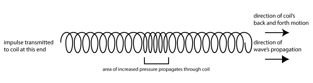
Sound waves are longitudinal waves. In a longitudinal wave, the displacement of the medium is parallel to the direction in which the wave propagates. For sound waves in air, air molecules are oscillating back and forth and propagating their energy in the same direction as their motion. You can picture a more concrete example if you remember the slinky toy of your childhood. If you and a friend lay a slinky along the floor and pull and push it back and forth, you create a longitudinal wave. The coils that make up the slinky are moving back and forth horizontally, in the same direction in which the wave propagates. The bouncing of a spring that is dangled vertically amounts to the same thing – a longitudinal wave.
[wpfilebase tag=file id=133 tpl=supplement /]
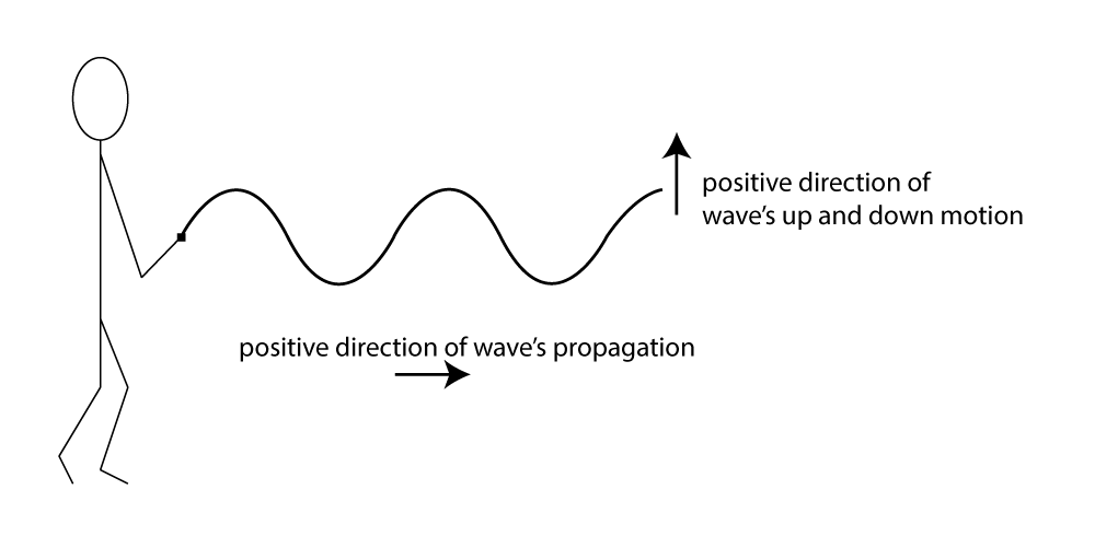
In contrast, in a transverse wave, the displacement of the medium is perpendicular to the direction in which the wave propagates. A jump rope shaken up and down is an example of a transverse wave. We call the quick shake that you give to the jump rope an impulse – like imparting a “bump” to the rope that propagates to the opposite end. The rope moves up and down, but the wave propagates from side to side, from one end of the rope to another. (You could also use your slinky to create a transverse wave, flipping it up and down rather than pushing and pulling it horizontally.)
2.1.4 Resonance
2.1.4.1 Resonance as Harmonic Frequencies
Have you ever heard someone use the expression, “That resonates with me”? A more informal version of this might be “That rings my bell.” What they mean by these expressions is that an object or event stirs something essential in their nature. This is a metaphoric use of the concept of resonance.
Resonance is an object’s tendency to vibrate or oscillate at a certain frequency that is basic to its nature. These vibrations can be excited in the presence of a stimulating force – like the ringing of a bell – or even in the presence of a frequency that sets it off – like glass shattering when just the right high-pitched note is sung. Musical instruments have natural resonant frequencies. When they are plucked, blown into, or struck, they vibrate at these resonant frequencies and resist others.
[wpfilebase tag=file id=107 tpl=supplement /]
Resonance results from an object’s shape, material, tension, and other physical properties. An object with resonance – for example, a musical instrument – vibrates at natural resonant frequencies consisting of a fundamental frequency and the related harmonic frequencies, all of which give an instrument its characteristic sound. The fundamental and harmonic frequencies are also referred to as the partials, since together they make up the full sound of the resonating object. The harmonic frequencies beyond the fundamental are called overtones. These terms can be slightly confusing. The fundamental frequency is the first harmonic because this frequency is one times itself. The frequency that is twice the fundamental is called the second harmonic or, equivalently, the first overtone. The frequency that is three times the fundamental is called the third harmonic or second overtone, and so forth. The number of harmonic frequencies depends upon the properties of the vibrating object.
One simple way to understand the sense in which a frequency might be natural to an object is to picture pushing a child on a swing. If you push a swing when it is at the top of its arc, you’re pushing it at its resonant frequency, and you’ll get the best effect with your push. Imagine trying to push the swing at any other point in the arc. You would simply be fighting against the natural flow. Another way to illustrate resonance is by means of a simple transverse wave, as we’ll show in the next section.
2.1.4.2 Resonance of a Transverse Wave
[wpfilebase tag=file id=130 tpl=supplement /]
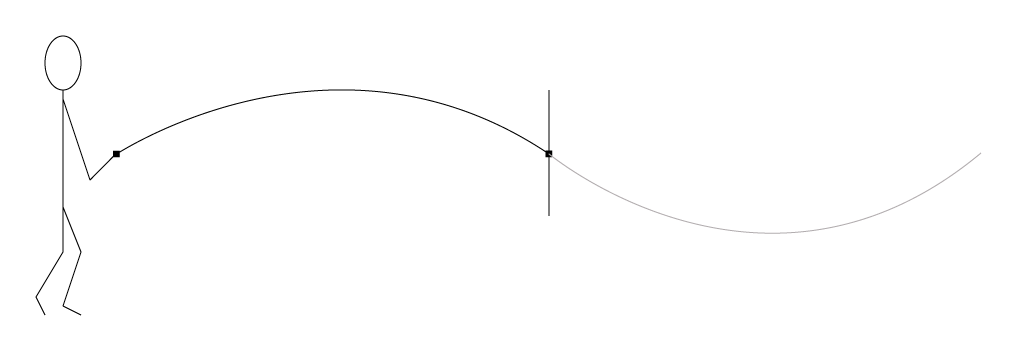
We can observe resonance in the example of a simple transverse wave that results from sending an impulse along a rope that is fixed at both ends. Imagine that you’re jerking the rope upward to create an impulse. The widest upward bump you could create in the rope would be the entire length of the rope. Since a wave consists of an upward movement followed by a downward movement, this impulse would represent half the total wavelength of the wave you’re transmitting. The full wavelength, twice the length of the rope, is conceptualized in Figure 2.9. This is the fundamental wavelength of the fixed-end transverse wave. The fundamental wavelength (along with the speed at which the wave is propagated down the rope) defines the fundamental frequency at which the shaken rope resonates.
[equation caption=”Equation 2.4″]If L is the length of a rope fixed at both ends, then λ is the fundamental wavelength of the rope, given by
$$!\lambda =2L$$
[/equation]
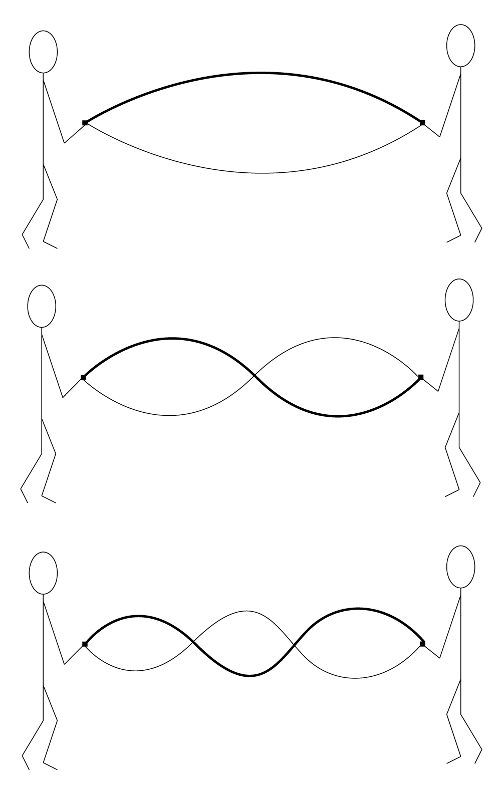
Now imagine that you and a friend are holding a rope between you and shaking it up and down. It’s possible to get the rope into a state of vibration where there are stationary points and other points between them where the rope vibrates up and down, as shown in Figure 2.10. This is called a standing wave. In order to get the rope into this state, you have to shake the rope at a resonant frequency. A rope can vibrate at more than one resonant frequency, each one giving rise to a specific mode – i.e., a pattern or shape of vibration. At its fundamental frequency, the whole rope is vibrating up and down (mode 1). Shaking at twice that rate excites the next resonant frequency of the rope, where one half of the rope is vibrating up while the other is vibrating down (mode 2). This is the second harmonic (first overtone) of the vibrating rope. In the third harmonic, the “up and down” vibrating areas constitute one third of the rope’s length each.
This phenomenon of a standing wave and resonant frequencies also manifests itself in a musical instrument. Suppose that instead of a rope, we have a guitar string fixed at both ends. Unlike the rope that is shaken at different rates of speed, guitar strings are plucked. This pluck, like an impulse, excites multiple resonant frequencies of the string at the same time, including the fundamental and any harmonics. The fundamental frequency of the guitar string results from the length of the string, the tension with which it is held between two fixed points, and the physical material of the string.
The harmonic modes of a string are depicted in Figure 2.11. The top picture in the figure illustrates the string vibrating according to its fundamental frequency. The wavelength l of the fundamental frequency is two times the length of the string L.
The second picture from the top in Figure 2.11 shows the second harmonic frequency of the string. Here, the wavelength is equal to the length of the string, and the corresponding frequency is twice the frequency of the fundamental. In the third harmonic frequency, the wavelength is 2/3 times the length of the string, and the corresponding frequency is three times the frequency of the fundamental. In the fourth harmonic frequency, the wavelength is 1/2 times the length of the string, and the corresponding frequency is four times the frequency of the fundamental. More harmonic frequencies could exist beyond this depending on the type of string.
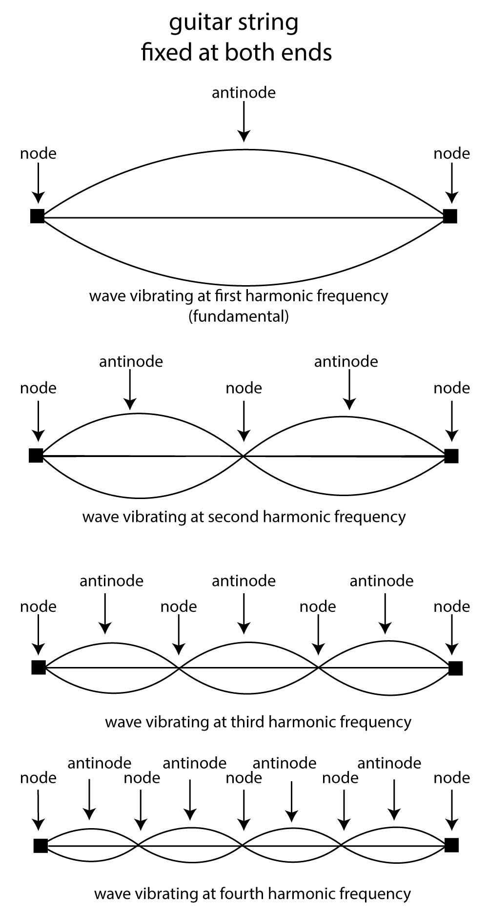
Like a rope held at both ends, a guitar string fixed at both ends creates a standing wave as it vibrates according to its resonant frequencies. In a standing wave, there exist points in the wave that don’t move. These are called the nodes, as pictured in Figure 2.11. The antinodes are the high and low points between which the string vibrates. This is hard to illustrate in a still image, but you should imagine the wave as if it’s anchored at the nodes and swinging back and forth between the nodes with high and low points at the antinodes.
It’s important to note that this figure illustrates the physical movement of the string, not a graph of a sine wave representing the string’s sound. The string’s vibration is in the form of a transverse wave, where the string moves up and down while the tensile energy of the string propagates perpendicular to the vibration. Sound is a longitudinal wave.
The speed of the wave’s propagation through the string is a function of the tension force on the string, the mass of the string, and the string’s length. If you have two strings of the same length and mass and one is stretched more tightly than another, it will have a higher wave propagation speed and thus a higher frequency. The frequency arises from the properties of the string, including its fundamental wavelength, 2L, and the extent to which it is stretched.
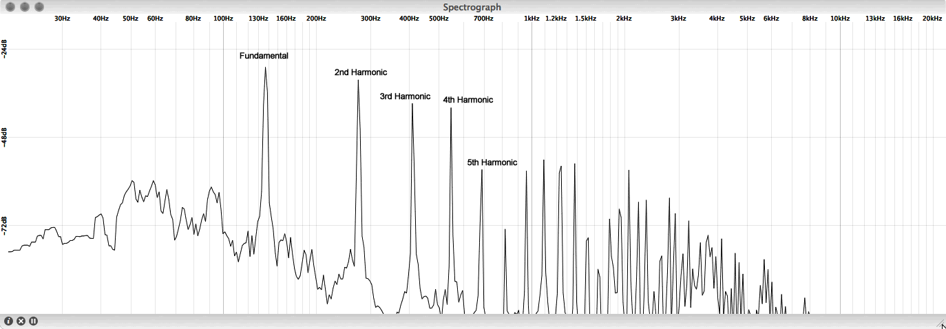
What is most significant is that you can hear the string as it vibrates at its resonant frequencies. These vibrations are transmitted to a resonant chamber, like a box, which in turn excites the neighboring air molecules. The excitation is propagated through the air as a transfer of energy in a longitudinal sound wave. The frequencies at which the string vibrates are translated into air pressure changes occurring with the same frequencies, and this creates the sound of the instrument. Figure 2.12 shows an example harmonic spectrum of a plucked guitar string. You can clearly see the resonant frequencies of the string, starting with the fundamental and increasing in integer multiples (twice the fundamental, three times the fundamental, etc.). It is interesting to note that not all the harmonics resonate with the same energy. Typically, the magnitude of the harmonics decreases as the frequency increases, where the fundamental is the most dominant. Also keep in mind that the harmonic spectrum and strength of the individual harmonics can vary somewhat depending on how the resonator is excited. How hard a string is plucked, or whether it is bowed or struck with a wooden stick or soft mallet, can have an effect on the way the object resonates and sounds.
2.1.4.3 Resonance of a Longitudinal Wave
[wpfilebase tag=file id=131 tpl=supplement /]
Not all musical instruments are made from strings. Many are constructed from cylindrical spaces of various types, like those found in clarinets, trombones, and trumpets. Let’s think of these cylindrical spaces in the abstract as a pipe.
A significant difference between the type of wave created from blowing air into a pipe and a wave created by plucking a string is that the wave in the pipe is longitudinal while the wave on the string is transverse. When air is blown into the end of a pipe, air pressure changes are propagated through the pipe to the opposite end. The direction in which the air molecules vibrate is parallel to the direction in which the wave propagates.
Consider first a pipe that is open at both ends. Imagine that a sudden pulse of air is sent through one of the open ends of the pipe. The air is at atmospheric pressure at both open ends of the pipe. As the air is blown into the end, the air pressure rises, reaching its maximum at the middle and falling to its minimum again at the other open end. This is shown in the top part of Figure 2.13. The figure shows that the resulting fundamental wavelength of sound produced in the pipe is twice the length of the pipe (similar to the guitar string fixed at both ends).

[wpfilebase tag=file id=13 tpl=supplement /]
The situation is different if the pipe is closed at the end opposite to the one into which it is blown. In this case, air pressure rises to its maximum at the closed end. The bottom part of Figure 2.13 shows that in this situation, the closed end corresponds to the crest of the fundamental wavelength. Thus, the fundamental wavelength is four times the length of the pipe.
Because the wave in the pipe is traveling through air, it is simply a sound wave, and thus we know its speed – approximately 1130 ft/s. With this information, we can calculate the fundamental frequency of both closed and open pipes, given their length.
[equation caption=”Equation 2.5″]Let L be the length of an open pipe, and let c be the speed of sound. Then the fundamental frequency of the pipe is.
$$!\frac{c}{2L}$$
[/equation]
[equation caption=”Equation 2.6″]Let L be the length of a closed pipe, and let c be the speed of sound. Then the fundamental frequency of the pipe is .
$$!\frac{c}{4L}$$
[/equation]
This explanation is intended to shed light on why each instrument has a characteristic sound, called its timbre. The timbre of an instrument is the sound that results from its fundamental frequency and the harmonic frequencies it produces, all of which are integer multiples of the fundamental. All the resonant frequencies of an instrument can be present simultaneously. They make up the frequency components of the sound emitted by the instrument. The components may be excited at a lower energy and fade out at different rates, however. Other frequencies contribute to the sound of an instrument as well, like the squeak of fingers moving across frets, the sound of a bow pulled across a string, or the frequencies produced by the resonant chamber of a guitar’s body. Instruments are also characterized by the way their amplitude changes over time when they are plucked, bowed, or blown into. The changes of amplitude are called the amplitude envelope, as we’ll discuss in a later section.
Resonance is one of the phenomena that gives musical instruments their characteristic sounds. Guitar strings alone do not make a very audible sound when plucked. However, when a guitar string is attached to a large wooden box with a shape and size that is proportional to the wavelengths of the frequencies generated by the string, the box resonates with the sound of the string in a way that makes it audible to a listener several feet away. Drumheads likewise do not make a very audible sound when hit with a stick. Attach the drumhead to a large box with a size and shape proportional to the diameter of the membrane, however, and the box resonates with the sound of that drumhead so it can be heard. Even wind instruments benefit from resonance. The wooden reed of a clarinet vibrating against a mouthpiece makes a fairly steady and quiet sound, but when that mouthpiece is attached to a tube, a frequency will resonate with a wavelength proportional to the length of the tube. Punching some holes in the tube that can be left open or covered in various combinations effectively changes the length of the tube and allows other frequencies to resonate.
2.1.5 Digitizing Sound Waves
In this chapter, we have been describing sound as continuous changes of air pressure amplitude. In this sense, sound is an analog phenomenon – a physical phenomenon that could be represented as continuously changing voltages. Computers require that we use a discrete representation of sound. In particular, when sound is captured as data in a computer, it is represented as a list of numbers. Capturing sound in a form that can be handled by a computer is a process called analog-to-digital conversion, whereby the amplitude of a sound wave is measured at evenly-spaced intervals in time – typically 44,100 times per second, or even more. Details of analog-to-digital conversion are covered in Chapter 5. For now, it suffices to think of digitized sound as a list of numbers. Once a computer has captured sound as a list of numbers, a whole host of mathematical operations can be performed on the sound to change its loudness, pitch, frequency balance, and so forth. We’ll begin to see how this works in the following sections.
2.2.1 Acoustics
In each chapter, we begin with basic concepts in Section 1 and give applications of those concepts in Section 2. One main area where you can apply your understanding of sound waves is in the area of acoustics. “Acoustics” is a large topic, and thus we have devoted a whole chapter to it. Please refer to Chapter 4 for more on this topic.
2.2.2 Sound Synthesis
Naturally occurring sound waves almost always contain more than one frequency. The frequencies combined into one sound are called the sound’s frequency components. A sound that has multiple frequency components is a complex sound wave. All the frequency components taken together constitute a sound’s frequency spectrum. This is analogous to the way light is composed of a spectrum of colors. The frequency components of a sound are experienced by the listener as multiple pitches combined into one sound.
To understand frequency components of sound and how they might be manipulated, we can begin by synthesizing our own digital sound. Synthesis is a process of combining multiple elements to form something new. In sound synthesis, individual sound waves become one when their amplitude and frequency components interact and combine digitally, electrically, or acoustically. The most fundamental example of sound synthesis is when two sound waves travel through the same air space at the same time. Their amplitudes at each moment in time sum into a composite wave that contains the frequencies of both. Mathematically, this is a simple process of addition.
[wpfilebase tag=file id=29 tpl=supplement /]
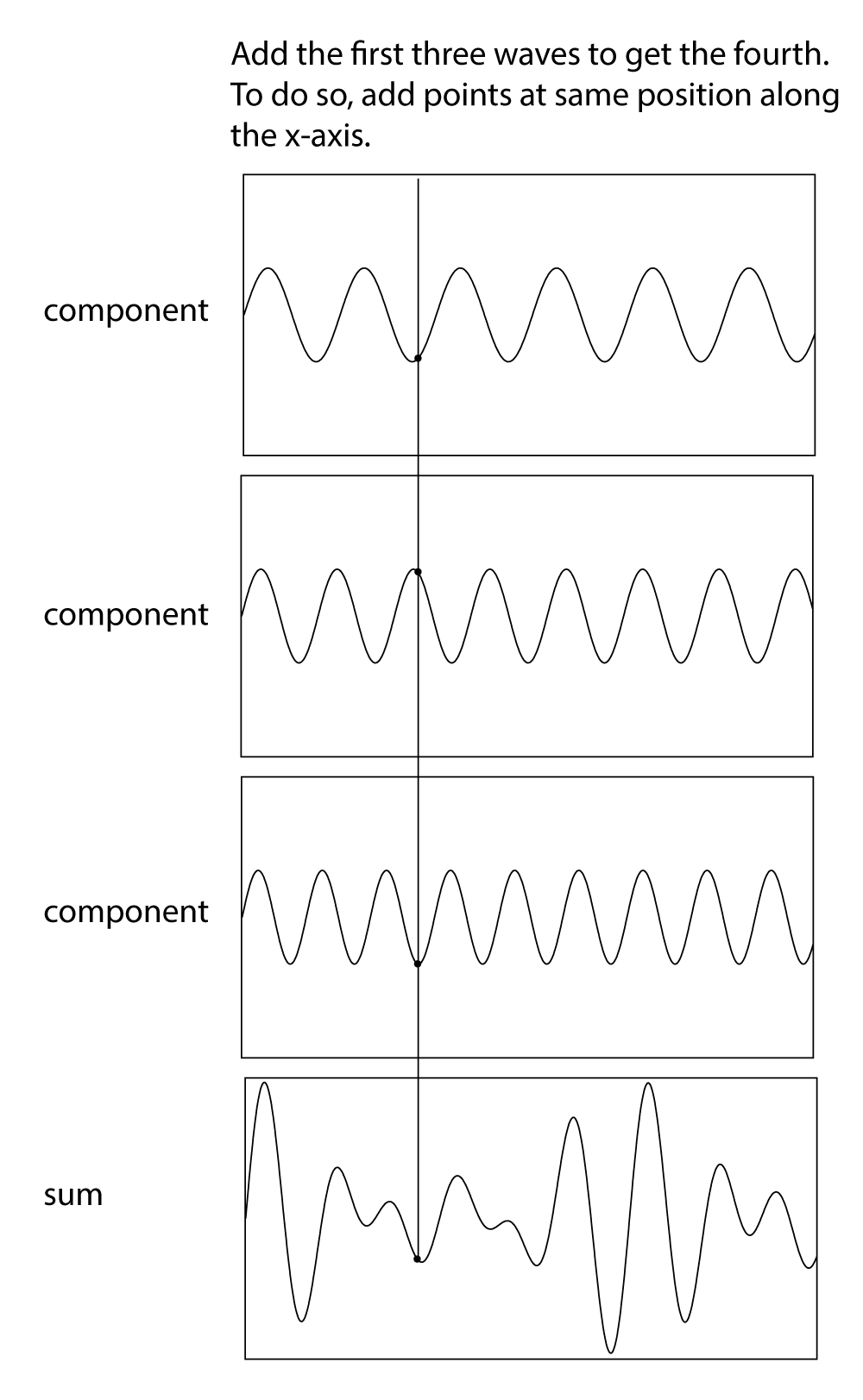
We can experiment with sound synthesis and understand it better by creating three single-frequency sounds using an audio editing program like Audacity or Adobe Audition. Using the “Generate Tone” feature in Audition, we’ve created three separate sound waves – the first at 262 Hz (middle C on a piano keyboard), the second at 330 Hz (the note E), and the third at 393 Hz (the note G). They’re shown in Figure 2.14, each on a separate track. The three waves can be mixed down in the editing software – that is, combined into a single sound wave that has all three frequency components. The mixed down wave is shown on the bottom track.
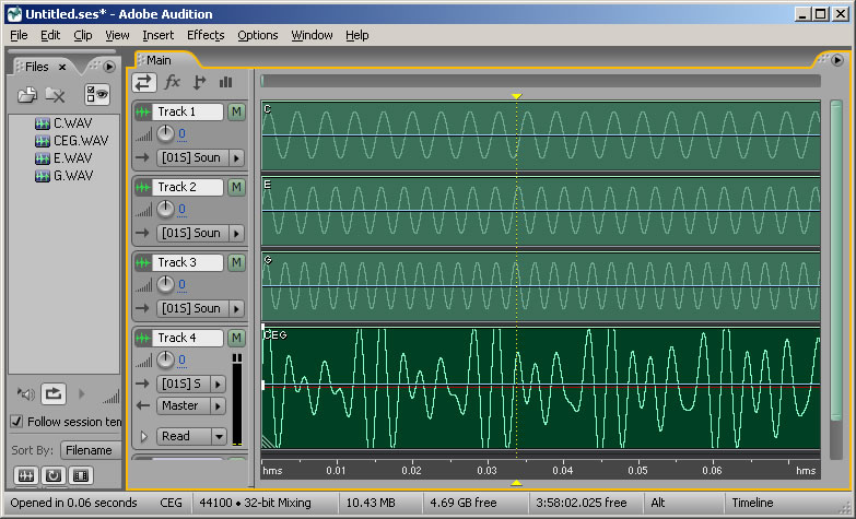
In a digital audio editing program like Audition, a sound wave is stored as a list of numbers, corresponding to the amplitude of the sound at each point in time. Thus, for the three audio tones generated, we have three lists of numbers. The mix-down procedure simply adds the corresponding values of the three waves at each point in time, as shown in Figure 2.15. Keep in mind that negative amplitudes (rarefactions) and positive amplitudes (compressions) can cancel each other out.
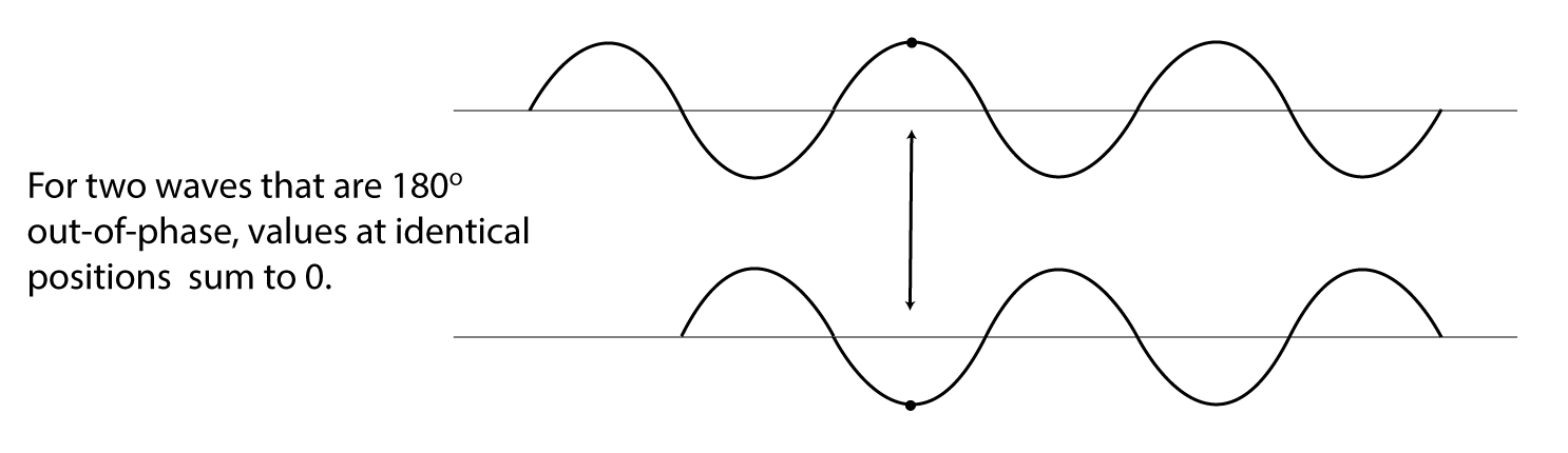
We’re able to hear multiple sounds simultaneously in our environment because sound waves can be added. Another interesting consequence of the addition of sound waves results from the fact that waves have phases. Consider two sound waves that have exactly the same frequency and amplitude, but the second wave arrives exactly one half cycle after the first – that is, 180o out-of-phase, as shown in Figure 2.16. This could happen because the second sound wave is coming from a more distant loudspeaker than the first. The different arrival times result in phase-cancellations as the two waves are summed when they reach the listener’s ear. In this case, the amplitudes are exactly opposite each other, so they sum to 0.
2.2.3 Sound Analysis
We showed in the previous section how we can add frequency components to create a complex sound wave. The reverse of the sound synthesis process is sound analysis, which is the determination of the frequency components in a complex sound wave. In the 1800s, Joseph Fourier developed the mathematics that forms the basis of frequency analysis. He proved that any periodic sinusoidal function, regardless of its complexity, can be formulated as a sum of frequency components. These frequency components consist of a fundamental frequency and the harmonic frequencies related to this fundamental. Fourier’s theorem says that no matter how complex a sound is, it’s possible to break it down into its component frequencies – that is, to determine the different frequencies that are in that sound, and how much of each frequency component there is.
[aside]”Frequency response” has a number of related usages in the realm of sound. It can refer to a graph showing the relative magnitudes of audible frequencies in a given sound. With regard to an audio filter, the frequency response shows how a filter boosts or attenuates the frequencies in the sound to which it is applied. With regard to loudspeakers, the frequency response is the way in which the loudspeakers boost or attenuate the audible frequencies. With regard to a microphone, the frequency response is the microphone’s sensitivity to frequencies over the audible spectrum.[/aside]
Fourier analysis begins with the fundamental frequency of the sound – the frequency of the longest repeated pattern of the sound. Then all the remaining frequency components that can be yielded by Fourier analysis – i.e., the harmonic frequencies – are integer multiples of the fundamental frequency. By “integer multiple” we mean that if the fundamental frequency is $$f_0$$ , then each harmonic frequency $$f_n$$ is equal to for some non-negative integer $$(n+1)f_0$$.
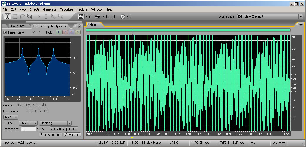
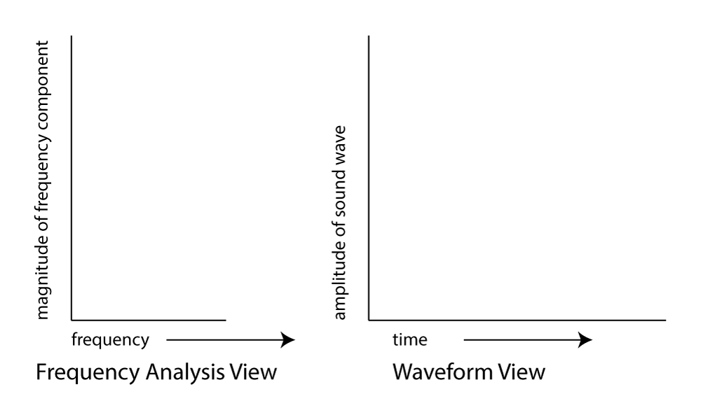
The Fourier transform is a mathematical operation used in digital filters and frequency analysis software to determine the frequency components of a sound. Figure 2.17 shows Adobe Audition’s waveform view and a frequency analysis view for a sound with frequency components at 262 Hz, 330 Hz, and 393 Hz. The frequency analysis view is to the left of the waveform view. The graph in the frequency analysis view is called a frequency response graph or simply a frequency response. The waveform view has time on the x-axis and amplitude on the y-axis. The frequency analysis view has frequency on the x-axis and the magnitude of the frequency component on the y-axis. (See Figure 2.18.) In the frequency analysis view in Figure 2.17, we zoomed in on the portion of the x-axis between about 100 and 500 Hz to show that there are three spikes there, at approximately the positions of the three frequency components. You might expect that there would be three perfect vertical lines at 262, 330, and 393 Hz, but this is because digitizing and transforming sound introduces some error. Still, the Fourier transform is accurate enough to be the basis for filters and special effects with sounds.
In the example just discussed, the frequencies that are combined in the composite sound never change. This is because of the way we constructed the sound, with three single-frequency waves that are held for one second. This sound, overall, is periodic because the pattern created from adding these three component frequencies is repeated over time, as you can see in the bottom of Figure 2.14.
Natural sounds, however, generally change in their frequency components as time passes. Consider something as simple as the word “information.” When you say “information,” your voice produces numerous frequency components, and these change over time. Figure 2.19 shows a recording and frequency analysis of the spoken word “information.”
When you look at the frequency analysis view, don’t be confused into thinking that the x-axis is time. The frequencies being analyzed are those that are present in the sound around the point in time marked by the yellow line.

In music and other sounds, pitches – i.e., frequencies – change as time passes. Natural sounds are not periodic in the way that a one-chord sound is. The frequency components in the first second of such sounds are different from the frequency components in the next second. The upshot of this fact is that for complex non-periodic sounds, you have to analyze frequencies over a specified time period, called a window. When you ask your sound analysis software to provide a frequency analysis, you have to set the window size. The window size in Adobe Audition’s frequency analysis view is called “FFT size.” In the examples above, the window size is set to 65536, indicating that the analysis is done over a span of 65,536 audio samples. The meaning of this window size is explained in more detail in Chapter 7. What is important to know at this point is that there’s a tradeoff between choosing a large window and a small one. A larger window gives higher resolution across the frequency spectrum – breaking down the spectrum into smaller bands – but the disadvantage is that it “blurs” its analysis of the constantly changing frequencies across a larger span of time. A smaller window focuses on what the frequency components are in a more precise, short frame of time, but it doesn’t yield as many frequency bands in its analysis.
2.2.4 Frequency Components of Non-Sinusoidal Waves
[wpfilebase tag=file id=108 tpl=supplement /]
In Section 2.1.3, we categorized waves by the relationship between the direction of the medium’s movement and the direction of the wave’s propagation. Another useful way to categorize waves is by their shape – square, sawtooth, and triangle, for example. These waves are easily described in mathematical terms and can be constructed artificially by adding certain harmonic frequency components in the right proportions. You may encounter square, sawtooth, and triangle waves in your work with software synthesizers. Although these waves are non-sinusoidal – i.e., they don’t take the shape of a perfect sine wave – they still can be manipulated and played as sound waves, and they’re useful in simulating the sounds of musical instruments.
A square wave rises and falls regularly between two levels (Figure 2.20, left). A sawtooth wave rises and falls at an angle, like the teeth of a saw (Figure 2.20, center). A triangle wave rises and falls in a slope in the shape of a triangle (Figure 2.20, right). Square waves create a hollow sound that can be adapted to resemble wind instruments. Sawtooth waves can be the basis for the synthesis of violin sounds. A triangle wave sounds very similar to a perfect sine wave, but with more body and depth, making it suitable for simulating a flute or trumpet. The suitability of these waves to simulate particular instruments varies according to the ways in which they are modulated and combined.

[aside]If you add the even numbered frequencies, you still get a sawtooth wave, but with double the frequency compared to the sawtooth wave with all frequency components.[/aside]
[wpfilebase tag=file id=11 tpl=supplement /]
Non-sinusoidal waves can be generated by computer-based tools – for example, Reason or Logic, which have built-in synthesizers for simulating musical instruments. Mathematically, non-sinusoidal waveforms are constructed by adding or subtracting harmonic frequencies in various patterns. A perfect square wave, for example, is formed by adding all the odd-numbered harmonics of a given fundamental frequency, with the amplitudes of these harmonics diminishing as their frequencies increase. The odd-numbered harmonics are those with frequency fn where f is the fundamental frequency and n is a positive odd integer. A sawtooth wave is formed by adding all harmonic frequencies related to a fundamental, with the amplitude of each frequency component diminishing as the frequency increases. If you would like to look at the mathematics of non-sinusoidal waves more closely, see Section 2.3.2.
[separator top=”1″ bottom=”0″ style=”none”]
2.2.5 Frequency, Impulse, and Phase Response Graphs
[aside]Although the term “impulse response” could technically be used for any instance of sound in the time domain, it is more often used to refer to instances of sound that are generated from a short burst of sound like a gun shot or balloon pop. In Chapter 7, you’ll see how an impulse response can be used to simulate the effect of an acoustical space on a sound.[/aside]
Section 2.2.3 introduces frequency response graphs, showing one taken from Adobe Audition. In fact, there are three interrelated graphs that are often used in sound analysis. Since these are used in this and later chapters, this is a good time to introduce you to these types of graphs. The three types of graphs are impulse response, frequency response, and phase response.
Impulse, frequency, and phase response graphs are simply different ways of storing and graphing the same set of data related to an instance of sound. Each type of graph represents the information in a different mathematical domain. The domains and ranges of the three types of sound graphs are given in Table 2.2.
[table caption=”Table 2.2 Domains and ranges of impulse, frequency, and phase response graphs” width=”80%”]
graph type,domain (x-axis),range (y-axis)
impulse response,time,amplitude of sound at each moment in time
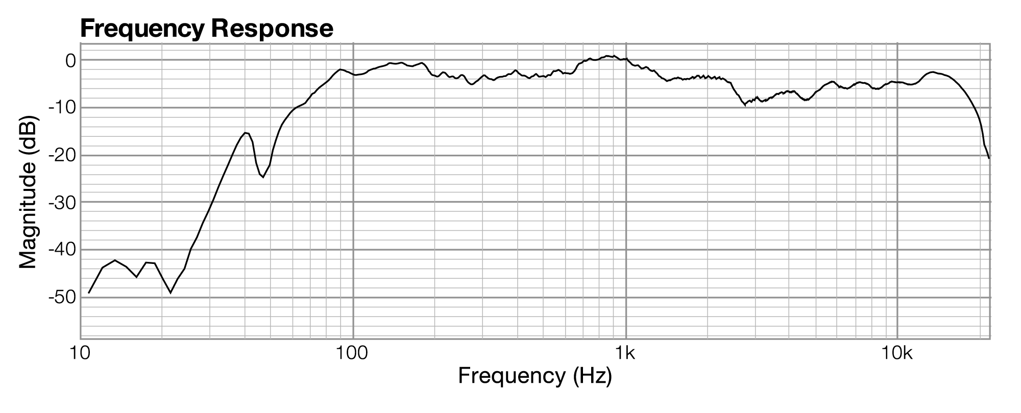
frequency response,frequency,magnitude of frequency across the audible spectrum of sound
phase response,frequency,phase of frequency across the audible spectrum of sound
[/table]
Let’s look at an example of these three graphs, each associated with the same instance of sound. The graphs in the figures below were generated by sound analysis software called Fuzzmeasure Pro.
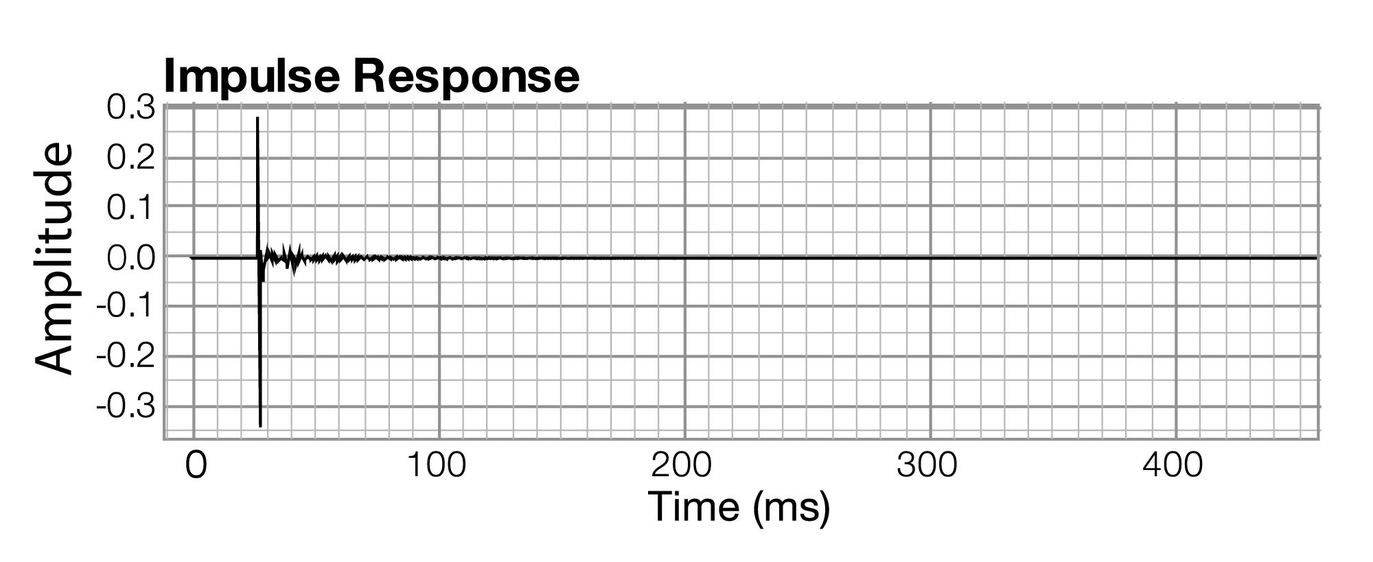

The impulse response graph shows the amplitude of the sound wave over time. The data used to draw this graph are produced by a microphone (and associated digitization hardware and software), which samples the amplitude of sound at evenly-spaced intervals of time. The details of this sound sampling process are discussed in Chapter 5. For now, all you need to understand is that when sound is captured and put into a form that can be handled by a computer, it is nothing more than a list of numbers, each number representing the amplitude of sound at a moment in time.
Related to each impulse response graph are two other graphs – a frequency response graph that shows “how much” of each frequency is present in the instance of sound, and a phase response graph that shows the phase that each frequency component is in. Each of these two graphs covers the audible spectrum. In Section 3, you’ll be introduced to the mathematical process – the Fourier transform – that converts sound data from the time domain to the frequency and phase domain. Applying a Fourier transform to impulse response data – i.e., amplitude represented in the time domain – yields both frequency and phase information from which you can generate a frequency response graph and a phase response graph. The frequency response graph has the magnitude of the frequency on the y-axis on whatever scale is chosen for the graph. The phase response graph has phases ranging from -180° to 180° on the y-axis.
The main points to understand are these:
- A graph is a visualization of data.
- For any given instance of sound, you can analyze the data in terms of time, frequency, or phase, and you can graph the corresponding data.
- These different ways of representing sound – as amplitude of sound over time or as frequency and phase over the audible spectrum – contain essentially the same information.
- The Fourier transform can be used to transform the sound data from one domain of representation to another. The Fourier transform is the basis for processes applied at the user-level in sound measuring and editing software.
- When you work with sound, you look at it and edit it in whatever domain of representation is most appropriate for your purposes at the time. You’ll see this later in examples concerning frequency analysis of live performance spaces, room modes, precedence effect, and so forth.