2.3.10 Windowing the FFT
When we applied the Fourier transform in MATLAB in Section 2.3.9, we didn’t specify a window size. Thus, we were applying the FFT to the entire piece of audio. If you listen to the WAV file HornsE04Mono.wav, a three second clip, you’ll first hear some low tubas and them some higher trumpets. Our graph of the FFT shows frequency components up to and beyond 5000 Hz, which reflects the sounds in the three seconds. What if we do the FFT on just the first second (44100 samples) of this WAV file, as follows? The resulting frequency components are shown in Figure 2.49.
y = audioread('HornsE04Mono.wav');
sr = 44100;
freqs = [0:(sr/2)-1];
ybegin = y(1:44100);
fftdata2 = fft(ybegin);
fftdata2 = fftdata2(1:22050);
plot(freqs, abs(fftdata2));
axis([0 5000 0 4500]);
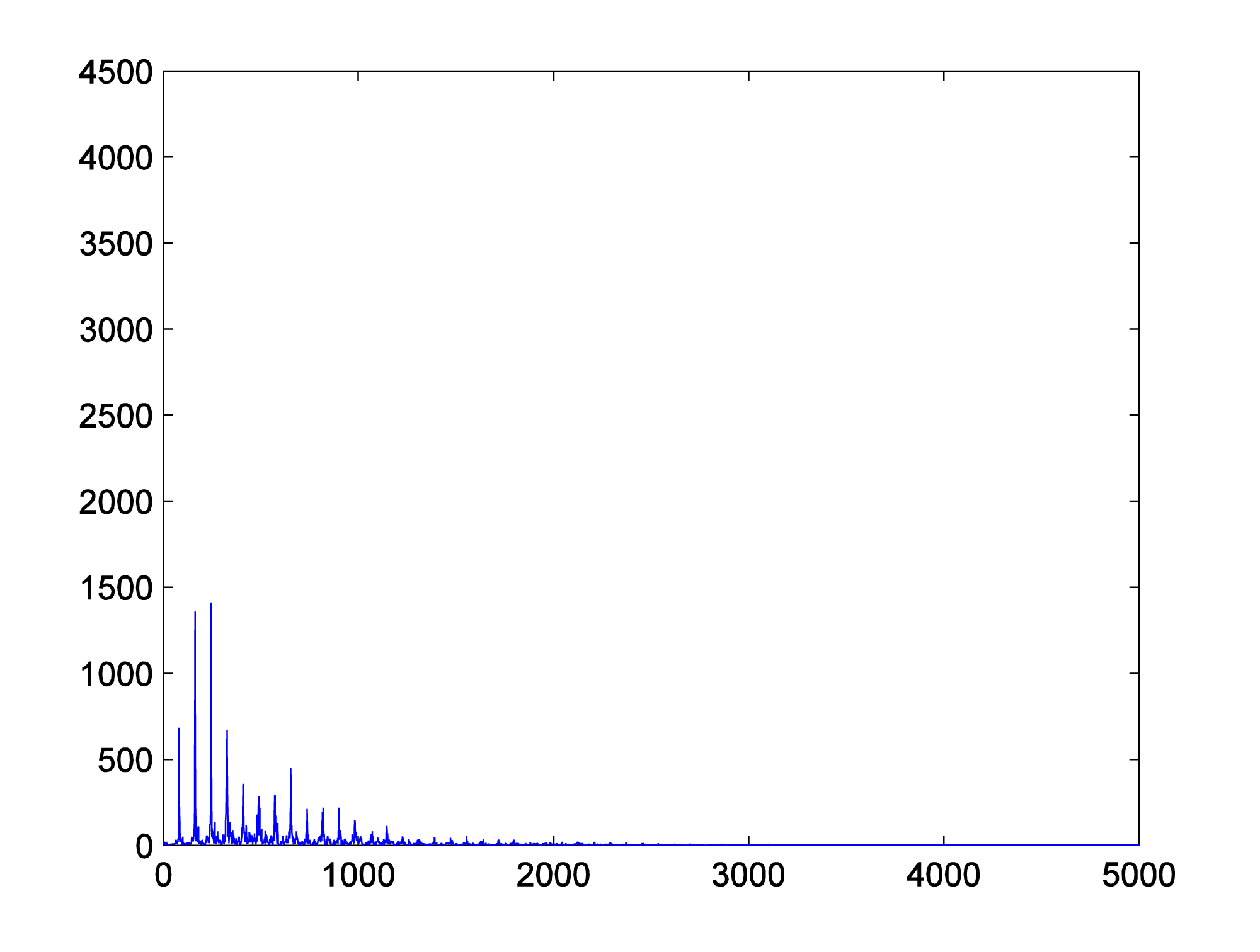
What we’ve done is focus on one short window of time in applying the FFT. An FFT window is a contiguous segment of audio samples on which the transform is applied. If you consider the nature of sound and music, you’ll understand why applying the transform to relatively small windows makes sense. In many of our examples in this book, we generate segments of sound that consist of one or more frequency components that do not change over time, like a single pitch note or a single chord being played without change. These sounds are good for experimenting with the mathematics of digital audio, but they aren’t representative of the music or sounds in our environment, in which the frequencies change constantly. The WAV file HornsE04Mono.wav serves as a good example. The clip is only three seconds long, but the first second is very different in frequencies (the pitches of tubas) from the last two seconds (the pitches of trumpets). When we do the FFT on the entire three seconds, we get a kind of “blurred” view of the frequency components, because the music actually changes over the three second period. It makes more sense to look at small segments of time. This is the purpose of the FFT window.
Figure 2.50 shows an example of how FFT window sizes are used in audio processing programs. Notice the drop down menu, which gives you a choice of FFT sizes ranging from 32 to 65536 samples. The FFT window size is typically a power of 2. If your sampling rate is 44,100 samples per second, then a window size of 32 samples is about 0.0007 s, and a window size of 65536 is about 1.486 s.
There’s a tradeoff in the choice of window size. A small window focuses on the frequencies present in the sound over a short period of time. However, as mentioned earlier, the number of frequency components yielded by an FFT of size N is N/2. Thus, for a window size of, say, 128, only 64 frequency bands are output, these bands spread over the frequencies from 0 Hz to sr/2 Hz where sr is the sampling rate. (See Chapter 5.) For a window size of 65536, 37768 frequency bands are output, which seems like a good thing, except that with the large window size, the FFT is not isolating a short moment of time. A window size of around 2048 usually gives good results. If you set the size to 2048 and play the piece of music loaded into Audition, you’ll see the frequencies in the frequency analysis view bounce up and down, reflecting the changing frequencies in the music as time pass.

2.3.11 Windowing Functions to Eliminate Spectral Leakage
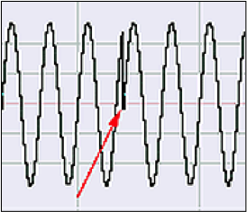
In addition to choosing the FFT window size, audio processing programs often let you choose from a number of windowing functions. The purpose of an FFT windowing function is to smooth out the discontinuities that result from applying the FFT to segments (i.e., windows) of audio data. A simplifying assumption for the FFT is that each windowed segment of audio data contains an integral number of cycles, this cycle repeating throughout the audio. This, of course, is not generally the case. If it were the case – that is, if the window ended exactly where the cycle ended – then the end of the cycle would be at exactly the same amplitude as the beginning. The beginning and end would “match up.” The actual discontinuity between the end of a window and its beginning is interpreted by the FFT as a jump from one level to another, as shown in Figure 2.51. (In this figure, we’ve cut and pasted a portion from the beginning of the window to its end to show that the ends don’t match up.)
In the output of the FFT, the discontinuity between the ends and the beginnings of the windows manifests itself as frequency components that don’t really exist in audio – called spurious frequencies, or spectral leakage. You can see the spectral leakage Figure 2.41. Although the audio signal actually contains only one frequency at 880 Hz, the frequency analysis view indicates that there is a small amount of other frequencies across the audible spectrum.
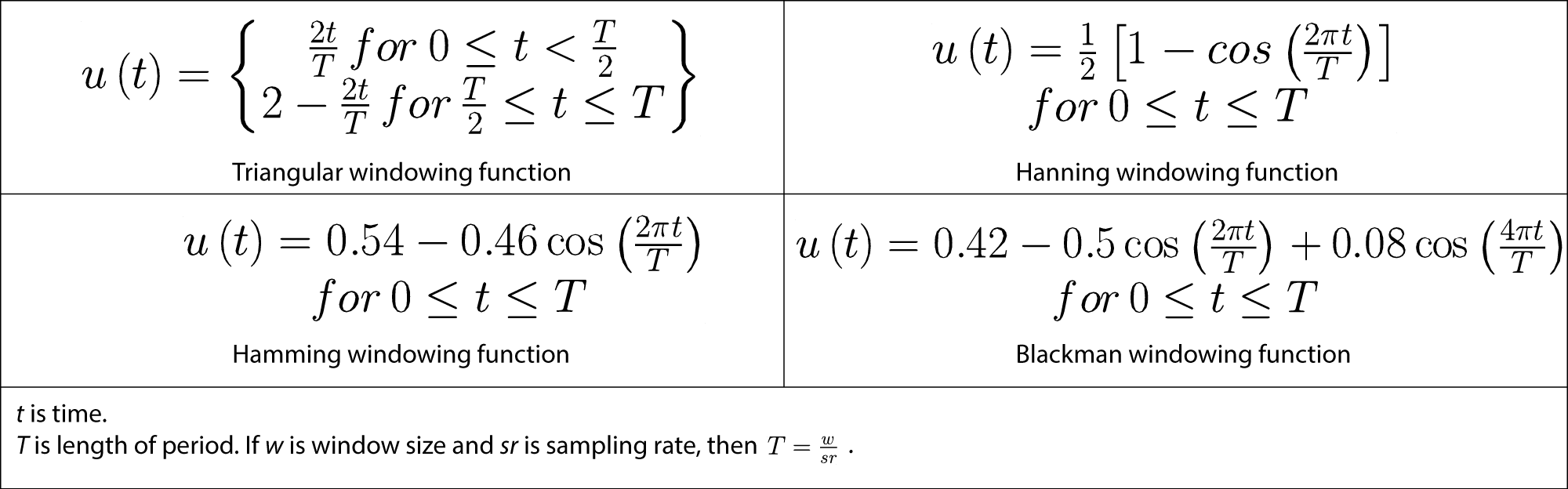
In order to smooth over this discontinuity and thereby reduce the amount of spectral leakage, the windowing functions effectively taper the ends of the segments to 0 so that they connect from beginning to end. The drop-down menu to the left of the FFT size menu in Audition is where you choose the windowing function. In Figure 2.50, the Hanning function is chosen. Four commonly-used windowing functions are given in the table below.
Windowing functions are easy to apply. The segment of audio data being transformed is simply multiplied by the windowing function before the transform is applied. In MATLAB, you can accomplish this with vector multiplication, as shown in the commands below.
y = audioread('HornsE04Mono.wav');
sr = 44100; %sampling rate
w = 2048; %window size
T = w/sr; %period
% t is an array of times at which the hamming function is evaluated
t = linspace(0, 1, 44100);
twindow = t(1:2048); %first 2048 elements of t
% Create the values for the hamming function, stored in vector called hamming
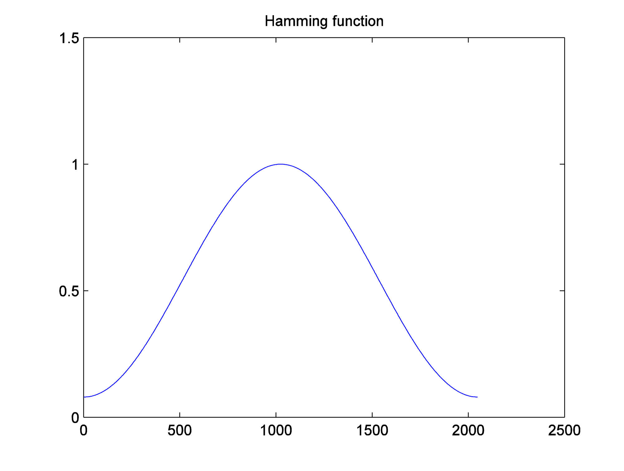
hamming = 0.54 - 0.46 * cos((2 * pi * twindow)/T);
plot(hamming);
title('Hamming');
The Hamming function is shown in
yshort = y(1:2048); %first 2048 samples from sound file
%Multiply the audio values in the window by the Hamming function values,
% using element by element multiplication with .*.
% first convert hamming from a column vector to a row vector
ywindowed = hamming .* yshort;
figure;
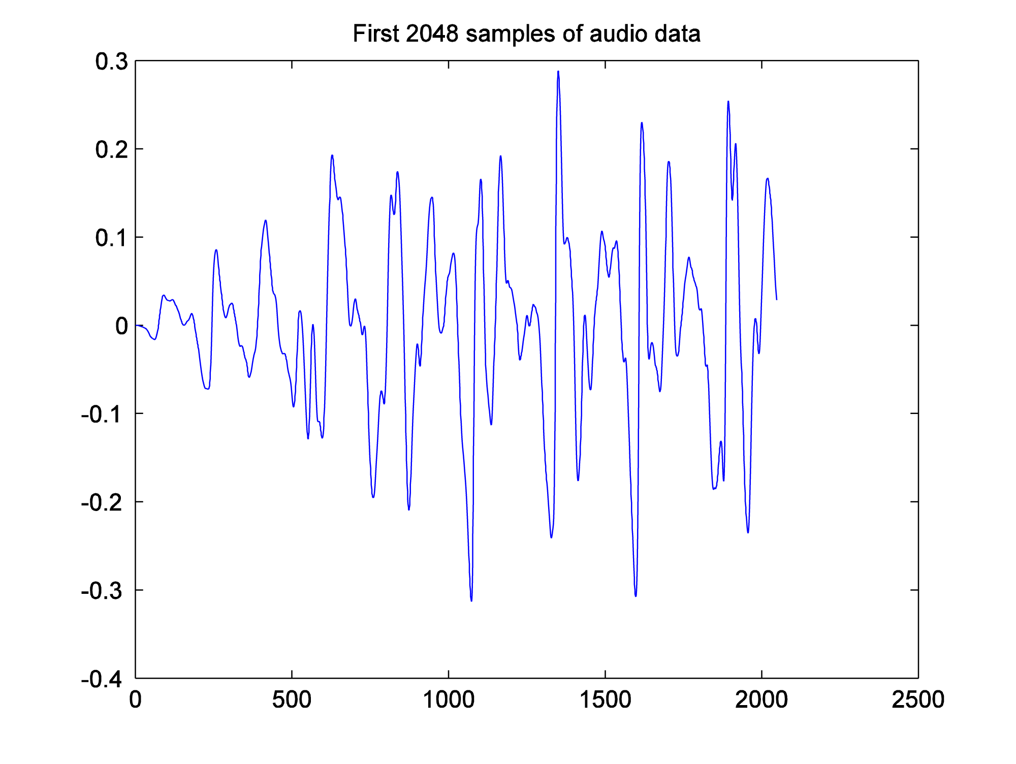
plot(yshort);
title('First 2048 samples of audio data');
figure;
plot(ywindowed);
title('First 2048 samples of audio data, tapered by windowing function');
Before the Hamming function is applied, the first 2048 samples of audio data look like this:
After the Hamming function is applied, the audio data look like this:
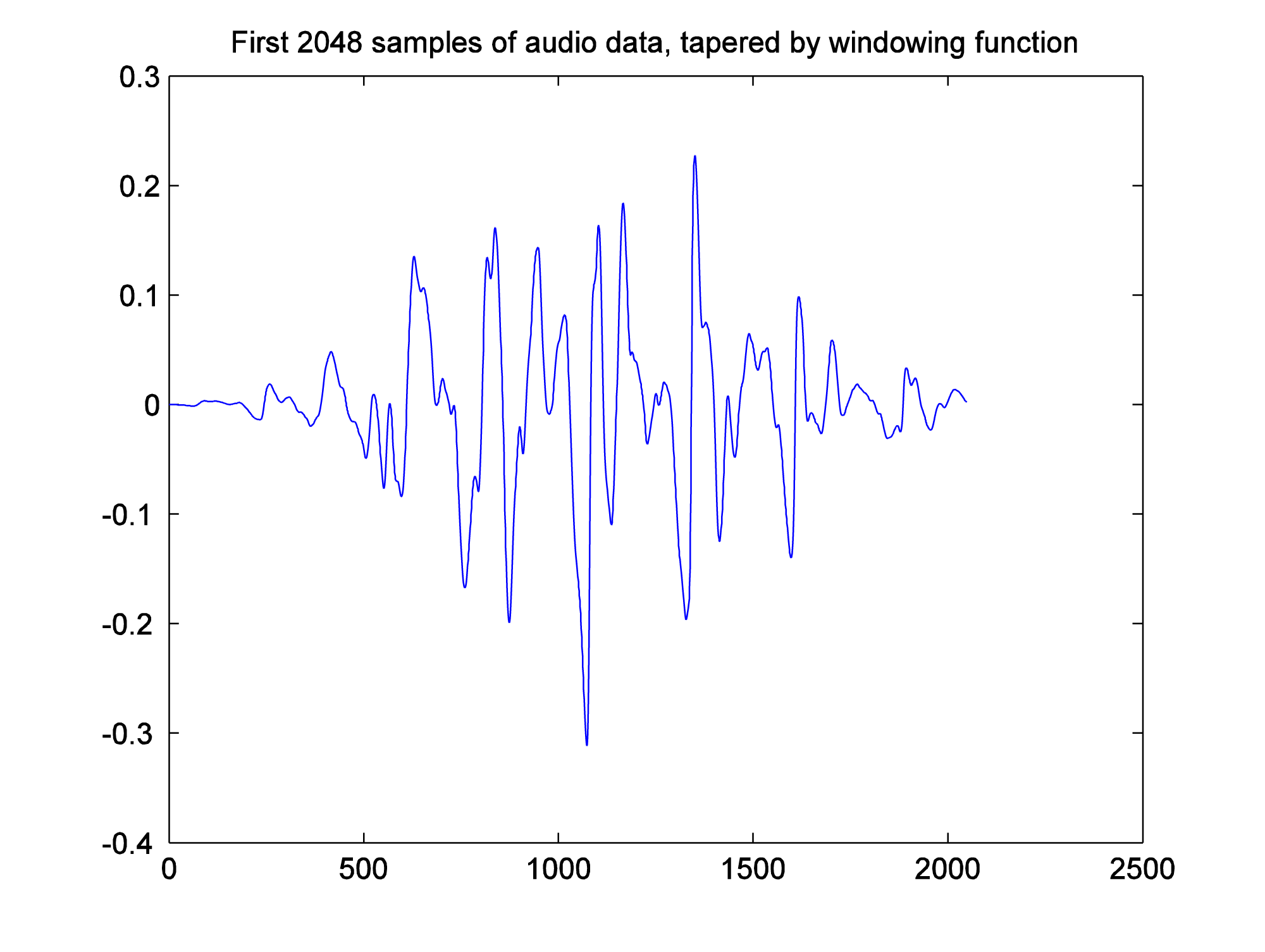
Notice that the ends of the segment are tapered toward 0.
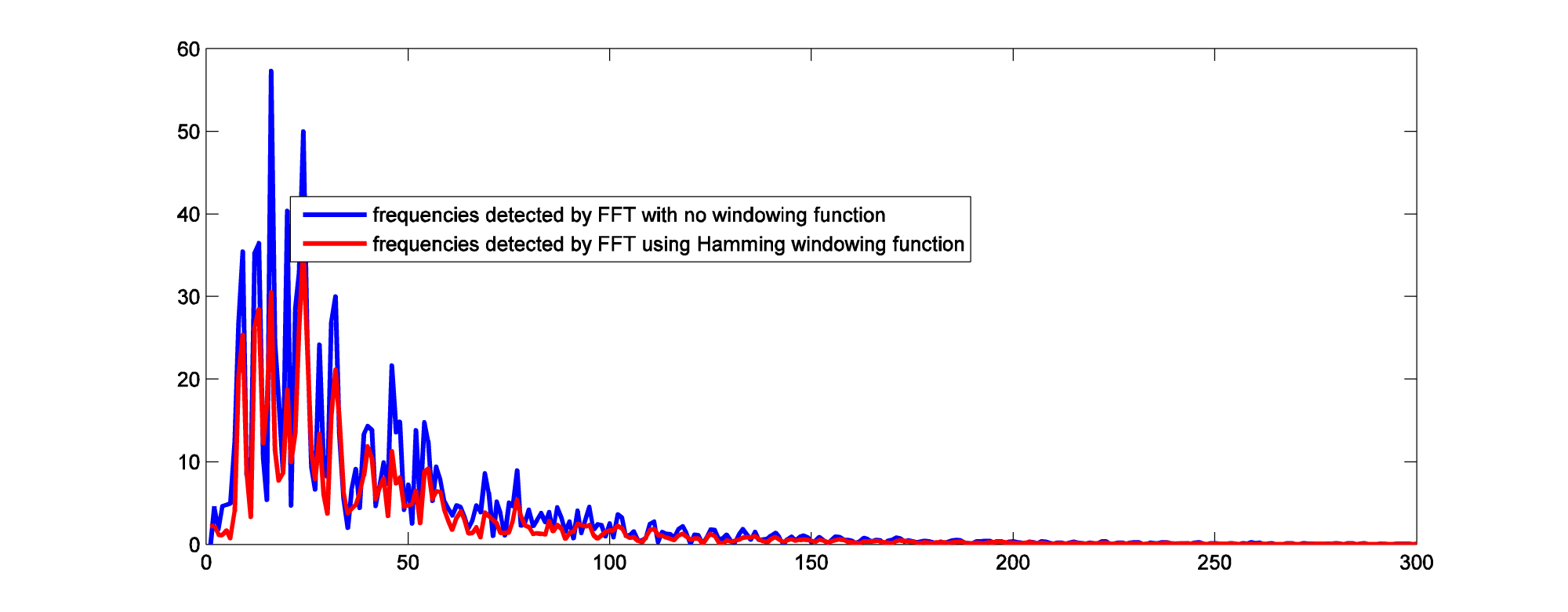
Figure 2.56 compares the FFT results with no windowing function vs. with the Hamming windowing function applied. The windowing function eliminates some of the high frequency components that are caused by spectral leakage.
figure
plot(abs(fft(yshort)));
axis([0 300 0 60]);
hold on;
plot(abs(fft(ywindowed)),'r');
[wpfilebase tag=file id=126 tpl=supplement /]
[separator top=”1″ bottom=”0″ style=”none”]
2.3.12 Modeling Sound in C++ under Linux
If you want to work at an even lower level of abstraction, a good environment for experimentation is the Linux operating system using “from scratch” programs written in C++. In our first example C++ sound program, we show you how to create sound waves of a given frequency, add frequency components to get a complex wave, and play the sounds via the sound device. This program is another implementation of the exercises in Max and MATLAB in Sections 2.3.1 and 2.3.3. The C++ program is given in Program 2.4. [aside]In this example program, 8 bits are used to store each audio sample. That is, the bit depth is 8. The sound library also allows a bit depth of 16. The concept of bit depth will be explained in detail in Chapter 5.
.[/aside]
//This program uses the OSS library.
#include <sys/ioctl.h> //for ioctl()
#include <math.h> //sin(), floor(), and pow()
#include <stdio.h> //perror
#include <fcntl.h> //open, O_WRONLY
#include <linux/soundcard.h> //SOUND_PCM*
#include <iostream>
#include <unistd.h>
using namespace std;

#define TYPE char
#define LENGTH 1 //number of seconds per frequency
#define RATE 44100 //sampling rate
#define SIZE sizeof(TYPE) //size of sample, in bytes
#define CHANNELS 1 //number of audio channels
#define PI 3.14159
#define NUM_FREQS 3 //total number of frequencies
#define BUFFSIZE (int) (NUM_FREQS*LENGTH*RATE*SIZE*CHANNELS) //bytes sent to audio device
#define ARRAYSIZE (int) (NUM_FREQS*LENGTH*RATE*CHANNELS) //total number of samples
#define SAMPLE_MAX (pow(2,SIZE*8 - 1) - 1)

void writeToSoundDevice(TYPE buf[], int deviceID) {
	int status;
	status = write(deviceID, buf, BUFFSIZE);
	if (status != BUFFSIZE)
		perror("Wrote wrong number of bytes\n");
	status = ioctl(deviceID, SNDCTL_DSP_SYNC, 0);
	if (status == -1)
		perror("SNDCTL_DSP_SYNC failed\n");
}

int main() {
	int deviceID, arg, status, f, t, a, i;
	TYPE buf[ARRAYSIZE];
	deviceID = open("/dev/dsp", O_WRONLY, 0);
	if (deviceID < 0)
		perror("Opening /dev/dsp failed\n");
// working
	arg = SIZE * 8;
	status = ioctl(deviceID, SNDCTL_DSP_SETFMT, &arg);
	if (status == -1)
		perror("Unable to set sample size\n");
	arg = CHANNELS;
	status = ioctl(deviceID, SNDCTL_DSP_CHANNELS, &arg);
	if (status == -1)
		perror("Unable to set number of channels\n");
	arg = RATE;
	status = ioctl(deviceID, SNDCTL_DSP_SPEED, &arg);
	if (status == -1)
		perror("Unable to set sampling rate\n");
	a = SAMPLE_MAX;
	for (i = 0; i < NUM_FREQS; ++i) {
		switch (i) {
			case 0:
				f = 262;
				break;
			case 1:
				f = 330;
				break;
			case 2:
				f = 392;
				break;
		}
		for (t = 0; t < ARRAYSIZE/NUM_FREQS; ++t) {
			buf[t + ((ARRAYSIZE / NUM_FREQS) * i)] = floor(a * sin(2*PI*f*t/RATE));
		}
	}
	writeToSoundDevice(buf, deviceID);
}
Program 2.4 Adding sine waves and sending sound to sound device in C++
To be able to compile and run a program such as this, you need to install a sound library in your Linux environment. At the time of the writing of this chapter, the two standard low-level sound libraries for Linux are the OSS (Open Sound System) and ALSA (Advanced Linux Sound Architecture). A sound library provides a software interface that allows your program to access the sound devices, sending and receiving sound data. ALSA is the newer of the two libraries and is preferred by most users. At a slightly higher level of abstraction are PulseAudio and Jack, applications which direct multiple sound streams from their inputs to their outputs. Ultimately, PulseAudio and Jack use lower level libraries to communicate directly with the sound cards.
[wpfilebase tag=file id=73 tpl=supplement /]
Program 2.4 uses the OSS library. In a program such as this, the sound device is opened, read from, and written to in a way similar to how files are handled. The sample program shows how you open /dev/dsp, an interface to the sound card device, to ask this device to receive audio data. The variable deviceID serves as an ID of the sound device and is used as a parameter indicating the size of data to expect, the number of channels, and the data rate. We’ve set a size of eight bits (one byte) per audio sample, one channel, and a data rate of 44,100 samples per second. The significance of these numbers will be clearer when we talk about digitization in Chapter 5. The buffer size is a product of the sample size, data rate, and length of the recording (in this case, three seconds), yielding a buffer of 44,100 * 3 bytes.
The sound wave is created by taking the sine of the appropriate frequency (262 Hz, for example) at 44,100 evenly-spaced intervals for one second of audio data. The value returned from the sine function is between -1 and 1. However, the sound card expects a value that is stored in one byte (i.e., 8 bits), ranging from -128 to 127. To put the value into this range, we multiply by 127 and, with the floor function, round down.
The three frequencies are created and concatenated into one array of audio values. The write function has the device ID, the name of the buffer for storing the sound data, and the size of the buffer as its parameters. This function sends the sound data to the sound card to be played. The three frequencies together produce a harmonious chord in the key of C. In Chapter 3, we’ll explore what makes these frequencies harmonious.
[wpfilebase tag=file id=75 tpl=supplement /]
The program requires some header files for definitions of constants like O_WRONLY (restricting access to the sound device to writing) and SOUND_PCM_WRITE_BITS. After you install the sound libraries, you’ll need to locate the appropriate header files and adjust the #include statement accordingly. You’ll also need to check the way your compiler handles the math and sound libraries. You may need to include the option –lm on the compile line to include the math library, or the –lasound option for the ALSA library.
This program introduces you to the notion that sound must be converted to a numeric format that is communicable to a computer. The solution to the programming assignment given as a learning supplement has an explanation of the variables and constants in this program. A full understanding of the program requires that you know something about sampling and quantization, the two main steps in analog-to-digital conversion, a topic that we’ll examine in depth in Chapter 5.
2.3.13 Modeling Sound in Java
The Java environment allows the programmer to take advantage of Java libraries for sound and to benefit from object-oriented programming features like encapsulation, inheritance, and interfaces. In this chapter, we are going to use the package javax.sound.sampled. This package provides functionality to capture, mix, and play sounds with classes such as SourceDataLine, AudioFormat, AudioSystem, and LineUnvailableException.
Program 2.5 uses a SourceDataLine object. This is the object to which we write audio data. Before doing that, we must set up the data line object with a specified audio format object. (See line 30.) The AudioFormat class specifies a certain arrangement of data in the sound stream, including the sampling rate, sample size in bits, and number of channels. A SourceDataLine object is created with the specified format, which in the example is 44,100 samples per second, eight bits per sample, and one channel for mono. With this setting, the line gets the required system resource and becomes operational. After the SourceDataLine is opened, data is written to the mixer using a buffer that contains data generated by a sine function. Notice that we don’t directly access the Sound Device because we are using a SourceDataLine object to deliver data bytes to the mixer. The mixer mixes the samples and finally delivers the samples to an audio output device on a sound card.
 import javax.sound.sampled.AudioFormat;
 import javax.sound.sampled.AudioSystem;
 import javax.sound.sampled.SourceDataLine;
 import javax.sound.sampled.LineUnavailableException;

 public class ExampleTone1{

   public static void main(String[] args){

     try {
         ExampleTone1.createTone(262, 100);
     } catch (LineUnavailableException lue) {
         System.out.println(lue);
     }
   }

   /** parameters are frequency in Hertz and volume
   **/
   public static void createTone(int Hertz, int volume)
     throws LineUnavailableException {
     /** Exception is thrown when line cannot be opened */

     float rate = 44100;
     byte[] buf;
     AudioFormat audioF;

     buf = new byte[1];
     audioF = new AudioFormat(rate,8,1,true,false);
     //sampleRate, sampleSizeInBits,channels,signed,bigEndian

     SourceDataLine sourceDL = AudioSystem.getSourceDataLine(audioF);
     sourceDL = AudioSystem.getSourceDataLine(audioF);
     sourceDL.open(audioF);
     sourceDL.start();

     for(int i=0; i<rate; i++){
       double angle = (i/rate)*Hertz*2.0*Math.PI;
       buf[0]=(byte)(Math.sin(angle)*volume);
       sourceDL.write(buf,0,1);
     }

     sourceDL.drain();
     sourceDL.stop();
     sourceDL.close();
   }
 }
Program 2.5 A simple sound generating program in Java
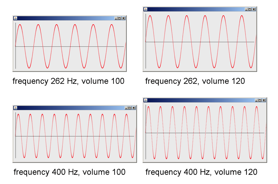
This program illustrates a simple of way of generating a sound by using a sine wave and the javax.sound.sampled library. If we change the values of the createTone procedure parameters, which are 262 Hz for frequency and 100 for volume, we can produce a different tone. The second parameter, volume, is used to change the amplitude of the sound. Notice that the sine function result is multiplied by the volume parameter in line 40.
Although the purpose of this section of the book is not to demonstrate how Java graphics classes are used, it may be helpful to use some basic plot features in Java to generate sine wave drawings. An advantage of Java is that it facilitates your control of windows and containers. We inherit this functionality from the JPanel class, which is a container where we are going to paint the sine wave generated. Program 2.6 is a variation of Program 2.5. It produces a Java Window by using the procedure paintComponent. This sine wave generated again has a frequency of 262 Hz and a volume of 100.
 import javax.sound.sampled.AudioFormat;
 import javax.sound.sampled.AudioSystem;
 import javax.sound.sampled.SourceDataLine;
 import javax.sound.sampled.LineUnavailableException;

 import java.awt.*;
 import java.awt.geom.*;
 import javax.swing.*;

 public class ExampleTone2 extends JPanel{

   static double[] sines;
   static int vol;

   public static void main(String[] args){

     try {
         ExampleTone2.createTone(262, 100);
     } catch (LineUnavailableException lue) {
         System.out.println(lue);
     }

     //Frame object for drawing
     JFrame frame = new JFrame();
     frame.setDefaultCloseOperation(JFrame.EXIT_ON_CLOSE);
     frame.add(new ExampleTone2());
     frame.setSize(800,300);
     frame.setLocation(200,200);
     frame.setVisible(true);
   }

   public static void createTone(int Hertz, int volume)
     throws LineUnavailableException {

     float rate = 44100;
     byte[] buf;
     buf = new byte[1];
     sines = new double[(int)rate];
     vol=volume;

     AudioFormat audioF;
     audioF = new AudioFormat(rate,8,1,true,false);

     SourceDataLine sourceDL = AudioSystem.getSourceDataLine(audioF);
     sourceDL = AudioSystem.getSourceDataLine(audioF);
     sourceDL.open(audioF);
     sourceDL.start();

     for(int i=0; i<rate; i++){
       double angle = (i/rate)*Hertz*2.0*Math.PI;
       buf[0]=(byte)(Math.sin(angle)*vol);
       sourceDL.write(buf,0,1);

       sines[i]=(double)(Math.sin(angle)*vol);
     }

     sourceDL.drain();
     sourceDL.stop();
     sourceDL.close();
   }

   protected void paintComponent(Graphics g) {
         super.paintComponent(g);
         Graphics2D g2 = (Graphics2D)g;
         g2.setRenderingHint(RenderingHints.KEY_ANTIALIASING,
                             RenderingHints.VALUE_ANTIALIAS_ON);

         int pointsToDraw=4000;
         double max=sines[0];
         for(int i=1;i<pointsToDraw;i++)  if (max<sines[i]) max=sines[i];
         int border=10;
         int w = getWidth();
         int h = (2*border+(int)max);

         double xInc = 0.5;

         //Draw x and y axes
         g2.draw(new Line2D.Double(border, border, border, 2*(max+border)));
         g2.draw(new Line2D.Double(border, (h-sines[0]), w-border, (h-sines[0])));

         g2.setPaint(Color.red);

         for(int i = 0; i < pointsToDraw; i++) {
             double x = border + i*xInc;
             double y = (h-sines[i]);
             g2.fill(new Ellipse2D.Double(x-2, y-2, 2, 2));
         }
    }
 }
Program 2.6 Visualizing the sound waves in a Java program
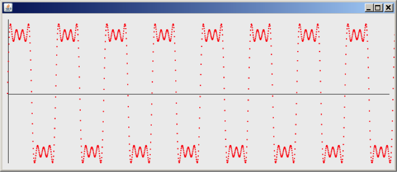
If we increase the value of the frequency in line 18 to 400 Hz, we can notice how the number of cycles increases, as shown in Figure 2.57. On the other hand, by increasing the volume, we obtain a higher amplitude for each frequency.
[wpfilebase tag=file id=77 tpl=supplement /]
We can also create square, triangle, and sawtooth waves in Java by modifying the for loop in lines 49 to 52. For example, to create a square wave, we may change the for loop to something like the following:
 for(int i=0; i<rate; i++){
   double angle1 = i/rate*Hertz*1.0*2.0*Math.PI;
   double angle2 = i/rate*Hertz*3.0*2.0*Math.PI;
   double angle3 = i/rate*Hertz*5.0*2.0*Math.PI;
   double angle4 = i/rate*Hertz*7.0*2.0*Math.PI;

   buf[0]=(byte)(Math.sin(angle1)*vol+
	Math.sin(angle2)*vol/3+Math.sin(angle3)*vol/5+
	Math.sin(angle4)*vol/7);
   sdl.write(buf,0,1);
   sines[i]=(double)(Math.sin(angle1)*vol+
	Math.sin(angle2)*vol/3+Math.sin(angle3)*vol/5+
	Math.sin(angle4)*vol/7);
 }
This for loop produces the sine wave shown in Figure 2.58. This graph doesn’t look like a perfect square wave, but the more harmonic frequencies we add, the closer we get to a square wave. (Note that you can create these waveforms more exactly by adapting the Octave programs above to Java.)
2.4 References
In addition to references cited in previous chapters:
Burg, Jennifer. The Science of Digital Media. Prentice-Hall, 2008.
Everest, F. Alton. Critical Listening Skills for Audio Professionals. Boston, MA: Course Technology CENGAGE Learning, 2007.
Jaffee, D. 1987. “Spectrum Analysis Tutorial, Part 1: The Discrete Fourier Transform. Computer Music Journal 11 (2): 9-24.
__________. 1987. “Spectrum Analysis Tutorial, Part 2: Properties and Applications of the Discrete Fourier Transform.” Computer Music Journal 11 (3): 17-35.
Kientzle, Tim. A Programmer’s Guide to Sound. Reading, MA: Addison-Wesley Developers Press, 1998.
Rossing, Thomas, F. Richard Moore, and Paul A. Wheeler. The Science of Sound. 3rd ed. San Francisco, CA: Addison-Wesley Developers Press, 2002.
Smith, David M. Engineering Computation with MATLAB. Boston: Pearson/Addison Wesley, 2008.
Steiglitz, K. A Digital Signal Processing Primer. Prentice-Hall, 1996.