Now let’s look at how the z-transform can be useful in describing, designing, and analyzing audio filters. We know that we can do filtering in the frequency domain with the operation
[equation caption=”Equation 7.7 Filtering in the frequency domain”]
$$!\mathbf{Y}\left ( z \right )=\mathbf{H}\left ( z \right )\ast \mathbf{X}\left ( z \right )$$
[/equation]
If we have the coefficients defining an FIR filter, $$\left [ a_{0},a_{1}.a_{2}\cdots ,a_{N-1} \right ]$$, then $$\mathbf{H}\left ( z \right )$$ is derived directly from the definition of the z-transform
[equation caption=”Equation 7.8 H(z), an FIR filter in the frequency domain”]
$$!\mathbf{H}\left ( z \right )=\sum_{n=0}^{N-1}\mathbf{h}\left ( n \right )z^{-n}=a_{0}+a_{1}z^{-1}+a_{2}z^{-2}+\cdots +a^{N-1}z^{-\left ( N-1 \right )}$$
[/equation]
Consider our previous example of an FIR filter,
$$!y\left ( n \right )=0.4x\left ( n \right )+0.3x\left ( n-1 \right )+0.3x\left ( n-2 \right )$$,
where $$\mathbf{h}=\left [ a_{0},a_{1},a_{2} \right ]=\left [ 0.4,0.3,0.3 \right ]$$. This filter can be transformed to the frequency domain by applying the z-transform.
$$!\mathbf{H}\left ( z \right )=\sum_{n=0}^{N-1}\mathbf{h}\left ( n \right )z^{-n}=a_{0}+a_{1}z^{-1}+a_{2}z^{-2}+\cdots +a^{N-1}z^{-\left ( N-1 \right )}=0.4+0.3z^{-1}+0.3z^{-2}$$
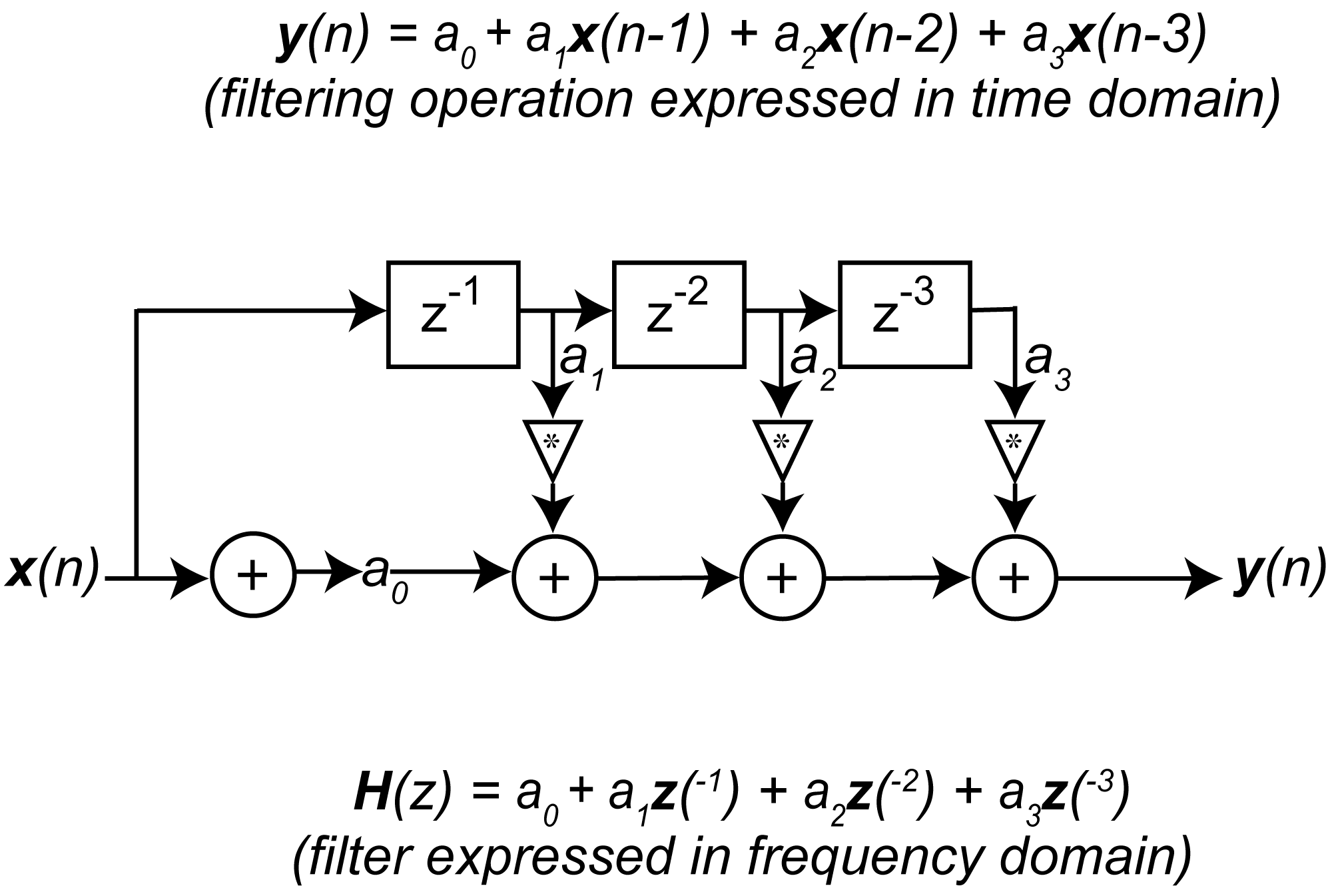
Filters can be expressed diagrammatically in terms of the z-transform, as illustrated in Figure 7.35. The $$z^{-m}$$ elements are delay elements.
To derive $$\mathbf{H}\left ( z \right )$$ for an IIR filter, we rearrange Equation 7.7 as a ratio of the output to the input.
[equation caption=”Equation 7.9 Filter in the frequency domain as a ratio of output to input”]
$$!\mathbf{H}\left ( z \right )=\frac{\mathbf{Y}\left ( z \right )}{\mathbf{X}\left ( z \right )}$$
[/equation]
This form of the filter is called the transfer function. Using the definition of the IIR filter, $$\mathbf{y}\left ( n \right )=\mathbf{h}\left ( n \right )\otimes \mathbf{x}\left ( n \right )=\sum_{k=0}^{N-1}a_{k}\mathbf{x}\left ( n-k \right )-\sum_{k=1}^{M}b_{k}\mathbf{y}\left ( n-k \right )$$, we can express the IIR filter in terms of its coefficients $$\left [ a_{0},a_{1},a_{2}\cdots ,a_{N-1} \right ]$$ and $$\left [ b_{1},b_{2},b_{3}\cdots ,b_{M} \right ]$$, which yields the following transfer function defining the IIR filter:
[equation caption=”Equation 7.10 Transfer function for an IIR filter”]
$$!\mathbf{H}\left ( z \right )=\frac{\mathbf{Y}\left ( z \right )}{\mathbf{X}\left ( z \right )}=\frac{a_{0}+a_{1}z^{-1}+a_{2}z^{-2}+\cdots +a_{N-1}z^{N-1}}{1+b_{1}z^{-1}+b_{2}z^{-2}+\cdots +b_{M}z^{N-M}}=\frac{a_{0}z^{N}+a_{1}z^{N-1}+\cdots +a_{N-1}z^{2N-1}}{z^{N}+b_{1}z^{N-1}+\cdots +b_{m}z^{2N-M}}$$
[/equation]
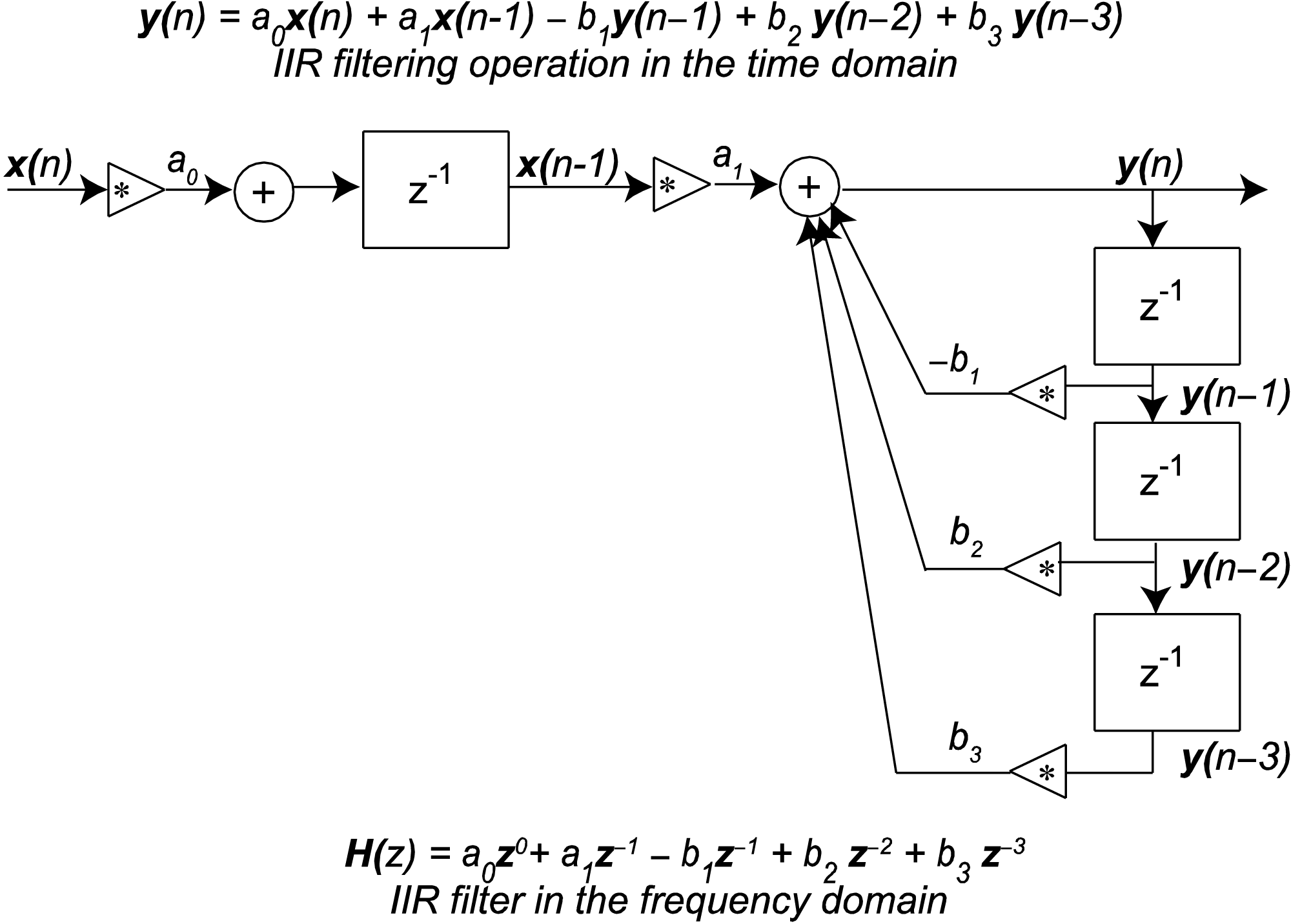
(The usefulness of transfer functions will become apparent in the next section.) An IIR filter in the frequency domain can be represented with a filter diagram as shown in Figure 7.36.
1 comment
Comments are closed.