In Chapter 2, we showed how the Fourier transform can be applied to transform audio data from the time to the frequency domain. The Fourier transform is a function that maps from real numbers (audio samples in the time domain) to complex numbers (frequencies, which have magnitude and phase). We showed in the previous section that the Fourier transform is a special case of the z-transform, a function that maps from complex numbers to complex numbers. Now let’s consider the equivalence of filtering in the time and frequency domains. We begin with some standard notation.
Say that you have a convolution filter as follows:
$$!\mathbf{y}\left ( n \right )=\mathbf{h}\left ( n \right )\otimes \mathbf{x}\left ( n \right )$$
By convention, the z-transform of $$\mathbf{x}\left ( n \right )$$ is called $$\mathbf{X}\left ( z \right )$$, the z-transform of $$\mathbf{y}\left ( n \right )$$is called $$\mathbf{Y}\left ( z \right )$$, and the z-transform of $$\mathbf{h}\left ( n \right )$$ is called $$\mathbf{H}\left ( z \right )$$, as shown in Table 7.1.
| time domain | frequency domain | |
| input audio | $$\mathbf{x}\left ( n \right )$$ | $$\mathbf{X}\left ( z \right )$$ |
| output, filtered audio | $$\mathbf{y}\left ( n \right )$$ | $$\mathbf{Y}\left ( z \right )$$ |
| filter | $$\mathbf{h}\left ( n \right )$$ | $$\mathbf{H}\left ( z \right )$$ |
| filter operation | $$\mathbf{y}\left ( n \right )=\mathbf{h}\left ( n \right )\otimes \mathbf{x}\left ( n \right )$$ | $$\mathbf{Y}\left ( z \right )=\mathbf{H}\left ( z \right )\ast \mathbf{X}\left ( z \right )$$ |
Table 7.1 Conventional notation for time and frequency domain filters
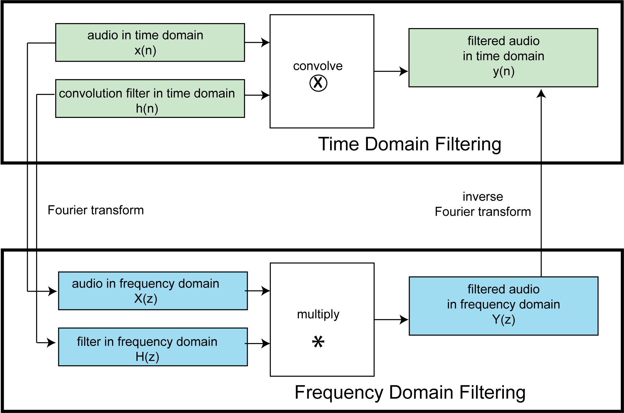
The convolution theorem is an important finding in digital signal processing that shows us the equivalence of filtering in the time domain vs. the frequency domain. By this theorem, instead of filtering by a convolution, as expressed in $$\mathbf{y}\left ( n \right )=\mathbf{h}\left ( n \right )\otimes \mathbf{x}\left ( n \right )$$, we can filter by multiplication, as expressed in $$\mathbf{Y}\left ( z \right )=\mathbf{H}\left ( z \right )\ast \mathbf{X}\left ( z \right )$$. (Note that $$\mathbf{H}\left ( z \right )\ast \mathbf{X}\left ( z \right )$$ is an element-by-element multiplication of order $$N$$.) That is, if you take a time domain filter, transform it to the frequency domain, transform your audio data to the frequency domain, multiply the frequency domain filter and the frequency domain audio data, and do the inverse Fourier transform on the result, you get the same result as you would get by convolving the time domain filter with the time domain audio data. This is in essence the convolution theorem, explained diagrammatically in Figure 7.34. In fact, with a fast implementation of the Fourier transform, known as the Fast Fourier Transform (FFT), filtering in the frequency domain is more computationally efficient than filtering in the time domain. That is, it takes less time to do the operations.
MATLAB has a function called fft for performing the Fourier transform on a vector of audio data and a function called conv for doing convolutions. However, to get a closer view of these operations, it may be enlightening to try implementing these functions yourself. You can implement the Fourier transform either directly from Equation 7.6, or you can try the more efficient algorithm, the Fast Fourier transform. To check your accuracy, you can compare your results with MATLAB’s functions. You can also compare the run times of programs that filter in the time vs. the frequency domain. We leave this as an activity for you to try.
In Chapter 2, we discussed the necessity of applying the Fourier transform over relatively small segments of audio data at a time. These segments, called windows, are on the order of about 1024 to 4096 samples. If you use the Fast Fourier transform, the window size must be a power of 2. It’s not hard to get an intuitive understanding of why the window has to be relatively small. The purpose of the Fourier transform is to determine the frequency components of a segment of sound. Frequency components relate to pitches that we hear. In most sounds, these pitches change over time, so the frequency components change over time. If you do the Fourier transform on, say, five seconds of audio, you’ll get an imprecise view of the frequency components in that time window, called time slurring. However, what if you choose a very small window size, say just one sample? You couldn’t possibly determine any frequencies in one sample, which at a sampling rate of 44.1 kHz is just 1/44,100 second. Frequencies are determined by how a sound wave’s amplitude goes up and down as time passes, so some time must pass for there to be such a thing as frequency.
The upshot of this observation is that the discrete Fourier transform has to be applied over windows of samples where the windows are neither too large nor too small. Note that the window size has a direct relationship with the number of frequency components you detect. If your window has a size of N, then you get an output telling you the magnitudes of N/2 frequency bands from the discrete Fourier transform, ranging in frequency from 0 to the Nyquist frequency (i.e., ½ the sampling rate). An overly small window in the Fourier transform gives you very high time resolution, but tells you the magnitudes of only a small number of discrete, wide bands of frequencies. An overly large window yields many frequency bands, but with poor time resolution that leads to slurring. You want to have good enough time resolution to be able to reconstruct the resulting audio signal, but also enough frequency information to apply the filters with proper effect. Choosing the right window size is a balancing act.