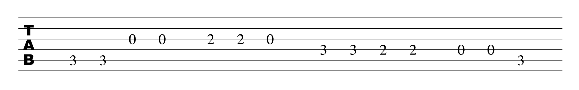
3.2.2 Tablature
Tablature (tab) is a common way of notating music when played on plucked string instruments. Basic guitar tablature requires that the player be somewhat familiar with the song already. As shown in Figure 3.43, guitar tabs use six lines like the regular music staff, but in this case, each line represents one of the six guitar strings. The top line represents the high E string and the bottom line represents the low E string. Numbers are then drawn on each line representing the fret number to use for that note on that string. To play the song, every time you see a number, you put your finger on that string at the fret number indicated and pluck that string. Simple tablature doesn’t give any indication of how long to play each note, so you need to be familiar with the song already. In some cases, the spacing of the numbers can give some indication of rhythm and duration.
3.2.3 Chord Progression
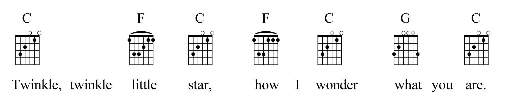
A common method for encoding musical data is with the chord progression. Consider the following chord progression for “Twinkle, Twinkle Little Star”:
[listtable width=”50%”]
- C F C
- Twinkle, twinkle little star
- F C G C
- How I wonder what you are.
- C F C G
- Up above the world so high,
- C F C G
- Like a diamond in the sky,
- C F C
- Twinkle, twinkle little star,
- F C G C
- How I wonder what you are.
[/listtable]
A trained musician who is already somewhat familiar with the tune should be able to extract the entire song as shown in Figure 3.37 from this chord progression. You may have witnessed an example of this if you’ve ever seen a live band that seemed able to play anything requested on the spur of the moment. Most good “gigging bands” can do this. Certainly, their ability to do this in part comes from a good familiarity with popular music, but that doesn’t mean they’ve memorized all those songs ahead of time. Musicians call this approach “faking it” and at most bookstores you can purchase “Fake Books” that contain hundreds of chord progressions for songs. With the musical data so highly compressed, it is not unheard of for a fake book to have well over 1000 songs in a size that can fit quite comfortably in a small backpack.
[wpfilebase tag=file id=35 tpl=supplement /]
In Section 3.1.6.2 we learned about intervals and in Section 3.1.6.3 we learned about chords. A chord progressions is a series of chords that underlie and support the melody of a song. Music is built with chord progressions. If you know what chord is being used at any given time in the song, you should also know which notes you could play for that part of the song. In the case of the chord progression for “Twinkle, Twinkle Little Star,” we begin with the tonic C major chord. Then we move to an F major chord. Occasionally, we use the G major chord. This is called a I-IV-V chord progression. Many popular songs are built from this chord progression. In the simplest form, you could play these chords on the keyboard as you sing the melody and you should have something that sounds familiar and harmonically satisfying. From there you could compose bass lines, solos, and arrangements by playing notes that fit with the key signature and chord currently in use. In addition to fake books, you can train your ears to recognize chord progressions and then fake the songs by ear. See the learning supplements for this section to start training your ears and try experimenting with improvising along with a chord progression.
3.2.4 Guitar Chord Grid
A guitar chord grid representation is of a chord sequence shown in Figure 3.44. The chord grid corresponds to the guitar fret board. The vertical lines represent the six strings and the horizontal lines represent the frets. A black dot represents a place on the fret board where you should put one of your fingers. When all your fingers are in the indicated locations, you can strum the strings to play the chord. Keep in mind that the chord grid shows you one way to play the chord, but there are always other fingering combinations that result in the same chord. If the grid you’re looking at looks too hard to play, you might be able to find a grid showing an alternate fingering that is easier.
3.3.2 Equal Tempered vs. Just Tempered Intervals
In Section 3.1.4 we described the diatonic scales that are commonly used in Western music. These scales are built by making the frequency of each successive note $$\sqrt[12]{2}$$ times the frequency of the previous one. This is just one example of a temperament, a system for selecting the intervals between tones used in musical composition. In particular, it is called equal temperament or equal tempered intonation, and it produces equal tempered scales and intervals. While this is the intonation our ears have gotten accustomed to in Western music, it isn’t the only one, nor even the earliest. In this section we’ll look at an alternative method for constructing scales that dates back to Pythagoras in the sixth century B. C. – just tempered intonation – a tuning in which frequency intervals are chosen based upon their harmonic relationships.
First let’s look more closely and the equal tempered scales as a point of comparison. The diatonic scales described in Section 3.1.4 are called equal tempered because the factor by which the frequencies get larger remains equal across the scale. Table 3.13 shows the frequencies of the notes from C4 to C5, assuming that A4 is 440 Hz. Each successive frequency is $$\sqrt[12]{2}$$ times the frequency of the previous one.
[table caption=”Table 3.13 Frequencies of notes from C4 to C5″ width=”30%”]
Note,Frequency
C4,261.63 Hz
C4# (D4♭),277.18Hz
D4,293.66 Hz
D4# (E4♭),311.13 Hz
E4,329.63 Hz
F4,349.23 Hz
F4# (G4♭),369.99 Hz
G4,392.00 Hz
G4# (A4♭),415.30 Hz
A4,440.00 Hz
A4# (B4♭),466.16 Hz
B4,493.88 Hz
C5,523.25 Hz
[/table]
It’s interesting to note how the ratio of two frequencies in an interval affects our perception of the interval’s consonance or dissonance. Consider the ratios of the frequencies for each interval type, as shown in Table 3.14. Some of these ratios reduce very closely to fractions with small integers in the numerator and denominator. For example, the frequencies of G and C, a perfect fifth, reduce to approximately 3:2; and the frequencies of E and C, a major third, reduce to approximately 5:4. Pairs of frequencies that reduce to fractions such as these are the ones that sound more consonant, as indicated in the last column of the table.
[table caption=”Table 3.14 Ratio of beginning and ending frequencies in intervals” width=”80%”]
Interval,Notes in Interval,Ratio of Frequencies,,Common Perception of Interval
perfect unison,C,261.63/261.63 ,1,consonant
minor second,C C#,277.18/261.63 ,≈ 1.059/1,dissonant
major second,C D,293.66/261.63 ,≈ 1.122/1,dissonant
minor third,C D E♭,311.13/261.63 ,≈ 1.189/1 ≈ 6/5,consonant
major third,C D E,329.63/261.63 ,≈ 1.260/1 ≈ 5/4,consonant
perfect fourth,C D E F,349.23/261.63 ,≈ 1.335/1 ≈ 4/3,strongly consonant
augmented fourth,C D E F#,369.99/261.63 ,≈ 1.414/1,dissonant
perfect fifth,C D E F G,392.00/261.63 ,≈ 1.498/1 ≈ 3/2,strongly consonant
minor sixth,C D E F G A♭,415.30/261.63 ,≈ 1.587/1 ≈ 8/5,consonant
major sixth,C D E F G A,440.00/261.63 ,≈ 1.681/1 ≈ 5/3,consonant
minor seventh,C D E F G A B♭,466.16/261.63 ,≈ 1.781/1,dissonant
major seventh,C D E F G A B ,493.88/261.63 ,≈ 1.887/1,dissonant
perfect octave,C C,523.26/261.63 ,1,consonant
[/table]
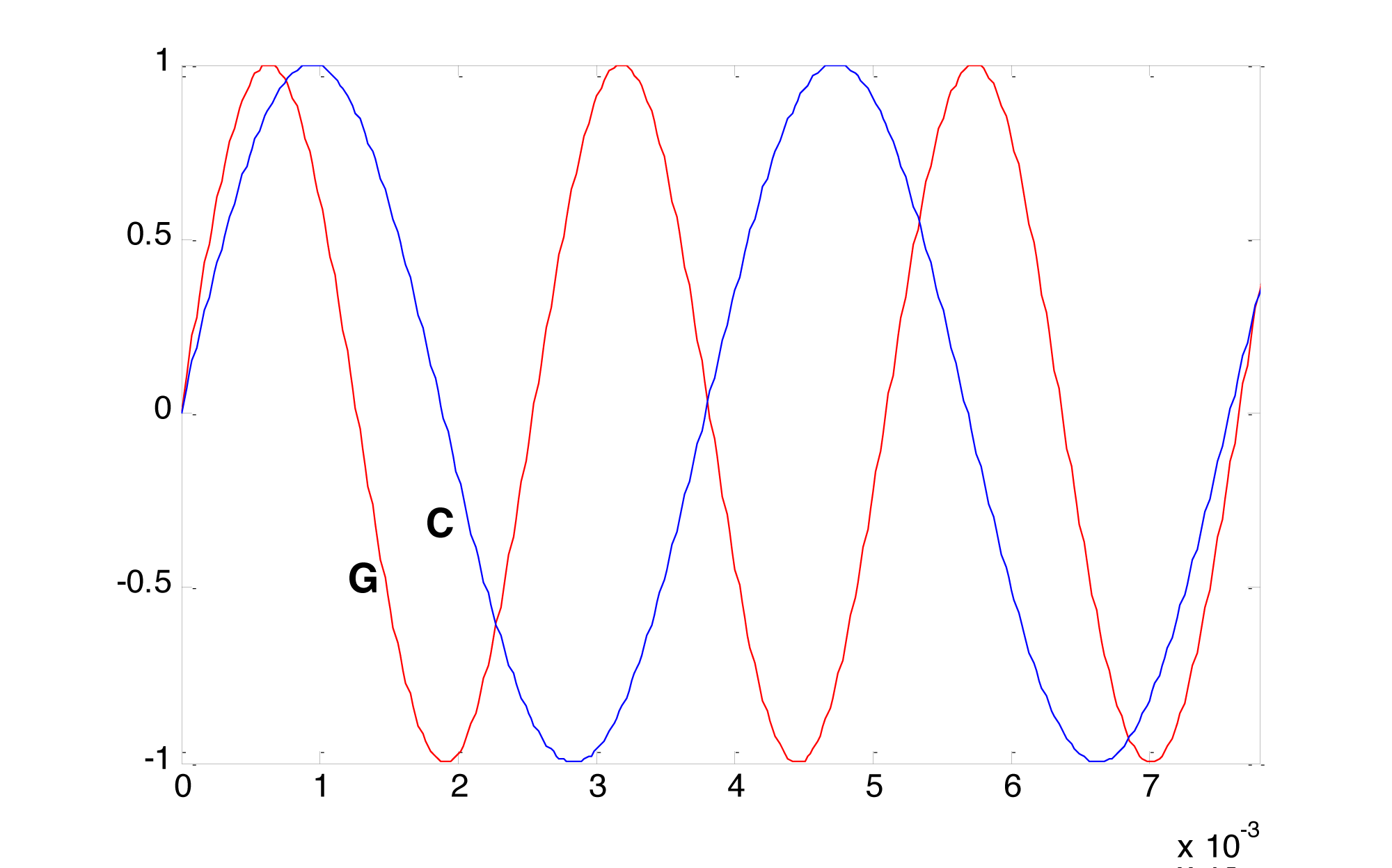
There’s a physical and mathematical explanation for this consonance. The fact that the frequencies of G and C have approximately a 3/2 ratio is visible in a graph of their sine waves. Figure 3.45 shows that three cycles of G fit almost exactly into two cycles of C. The sound waves fit together in an orderly pattern, and the human ear notices this agreement. But notice that we said the waves fit together almost exactly. The ratio of 392/261.63 is actually closer to 1.4983, not exactly 3/2, which is 1.5. Wouldn’t the intervals be even more harmonious if they were built upon the frequency relationships of natural harmonics?
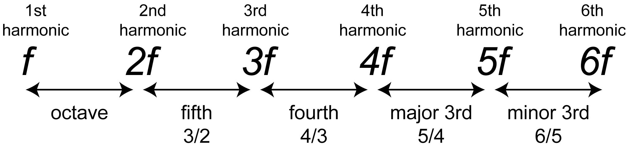
To consider how and why this might make sense, recall the definition of harmonic frequencies from Chapter 2. For a fundamental frequency $$f$$, the harmonic frequencies are $$1f$$, $$2f$$, $$3f$$, $$4f$$, and so forth. These are frequencies whose cycles do fit together exactly. As depicted in Figure 3.46, the ratio of the third to the second harmonic is $$\frac{3f}{2f}=\frac{3}{2}$$. This corresponds very closely, but not precisely, to what we have called a perfect fifth in equal tempered intonation – for example, the relationship between G and C in the key of C, or between D and G in the key of G. Similarly, the ratio of the fifth harmonic to the fourth is $$\frac{5f}{4f}=\frac{5}{4}$$, which corresponds to the interval we have referred to as a major third.
Just tempered intonations use frequencies that have these harmonic relationships. The Pythagoras diatonic scale is built entirely from fifths. The just tempered scale shown in Table 3.15 is a modern variant of Pythagoras’s scale. By comparing columns three and four, you can see how far the equal tempered tones are from the harmonic intervals. An interesting exercise would be to play a note in equal tempered frequency and then in just tempered frequency and see if you can notice the difference.
[table caption=”Table 3.15 Equal tempered vs. just tempered scales” width=”80%”]
Interval,Notes in Interval,Ratio of Frequencies in Equal Temperament,Ratio of Frequencies in Just Temperament
perfect unison,C,261.63/261.63 = 1.000,1/1 = 1.000
minor second,C C#,277.18/261.63 ≈ 1.059,16/15 ≈ 1.067
major second,C D,293.66/261.63 ≈ 1.122,9/8 = 1.125
minor third,C D E_,311.13/261.63 ≈ 1.189,6/5 = 1.200
major third,C D E,329.63/261.63 ≈ 1.260,5/4 ≈ 1.250
perfect fourth,C D E F,349.23/261.63 ≈ 1.335,4/3 ≈ 1.333
augmented fourth,C D E F#,369.99/261.63 ≈ 1.414,7/5 = 1.400
perfect fifth,C D E F G,392.00/261.63 ≈ 1.498,3/2 = 1.500
minor sixth,C D E F G A♭,415.30/261.63 ≈ 1.587,8/5 = 1.600
major sixth,C D E F G A,440.00/261.63 ≈ 1.682,5/3 ≈ 1.667
minor seventh,C D E F G A B♭,466.16/261.63 ≈ 1.782,7/4 = 1.750
major seventh,C D E F G A B ,493.88/261.63 ≈ 1.888,15/8 = 1.875
perfect octave,C C,523.26/261.63 = 2.000,2/1 = 2.000
[/table]
3.3.4 Experimenting with Music in MATLAB
Chapter 2 introduces some command line arguments for evaluating sine waves, playing sounds, and plotting graphs in MATLAB. For this chapter, you may find it more convenient to write functions in an external program. Files that contain code in the MATLAB language are called M-files, ending in the .m suffix. Here’s how you proceed when working with M-files:
- Create an M-file using MATLAB’s built-in text editor (or any text editor)
- Write a function in the M-file.
- Name the M-file fun1.m where fun1 is the name of function in the file.
- Place the M-file in your current MATLAB directory.
- Call the function from the command line, giving input arguments as appropriate and accepting the output by assigning it to a variable if necessary.
[wpfilebase tag=file id=53 tpl=supplement /]
The M-file can contain internal functions that are called from the main function. We refer you to MATLAB’s Help for details of syntax and program structure, but offer the program in Algorithm 3.1 to get you started. This program allows the user to create major and minor scales beginning with a start note. The start note is represented as a number of semitones offset from middle C. The function plays eight seconds of sound at a sampling rate of 44,100 samples per second and returns the raw data to the user, where it can be assigned to a variable on the command line if desired.
function outarray = MakeScale(startnoteoffset, isminor)
%outarray is an array of sound samples on the scale of (-1,1)
%outarray contains the 8 notes of a diatonic musical scale
%each note is played for one second
%the sampling rate is 44100 samples/s
%startnoteoffset is the number of semitones up or down from middle C at
%which the scale should start.
%If isminor == 0, a major scale is played; otherwise a minor scale is played.
sr = 44100;
s = 8;
outarray = zeros(1,sr*s);
majors=[0 2 4 5 7 9 11 12];
minors=[0 2 3 5 7 8 10 12];
if(isminor == 0)
    scale = majors;
else
    scale = minors;
end
scale = scale/12;
scale = 2.^scale;
%.^ is element-by-element exponentiation
t = [1:sr]/sr;
%the statement above is equivalent to
startnote = 220*(2^((startnoteoffset+3)/12))
scale = startnote * scale;
%Yes, ^ is exponentiation in MATLAB, rather than bitwise XOR as in C++
for i = 1:8
    outarray(1+(i-1)*sr:sr*i) = sin((2*pi*scale(i))*t);
end
 sound(outarray,sr);
Algorithm 3.1 Generating scales
The variables majors and minors hold arrays of integers, which can be created in MATLAB by placing the integers between square brackets, with no commas separating them. This is useful for defining, for each note in a diatonic scale, the number of semitones that the note is away from the key note.
[wpfilebase tag=file id=55 tpl=supplement /]
The lineThe variable scale is also an array, the same length as majors and minors (eight elements, because eight notes are played for the diatonic scale). Say that a major scale is to be created. Each element in scale is set to $$2^{\frac{majors\left [ i \right ]}{12}}$$, where majors[i] is the original value of element i in the array majors. (Note that arrays are numbered beginning at 1 in MATLAB.) This sets scale equal to $$\left [ 1,2^{\frac{2}{12}},2^{\frac{4}{12}},2^{\frac{5}{12}},2^{\frac{7}{12}},2^{\frac{9}{12}},2^{\frac{11}{12}} \right ]$$. When the start note is multiplied by each of these numbers, one at a time, the frequencies of the notes in a scale are produced.
x = [1:sr]/sr;
creates an array of 44,100 points between 0 and 1 at which the sine function is evaluated. (This is essentially equivalent to x = linspace(0,1, sr), which we used in previous examples.)
A3 with a frequency of 220 Hz is used as a reference point from which all other frequencies are built. Thus
startnote = 220*(2^((startnoteoffset+3)/12));
sets the start note to be middle C plus the user-defined offset.
In the for loop that repeats for eight seconds, the statement
outarray(1+(i-1)*sr:sr*i) = sin((2*pi*scale(i))*t);
writes the sound data into the appropriate section of outarray. It generates these samples by evaluating a sine function of the appropriate frequency across the 44,100-element array x. This statement is an example of how conveniently MATLAB handles array operations. A single call to a sine function can be used to evaluate the function over an entire array of values. The statement
scale = scale/12;
works similarly, dividing each element in the array scale by 12. The statement
scale = 2.^scale;
is also an element-by-element array operation, but in this case a dot has to be added to the exponentiation operator since ^ alone is matrix exponentiation, which can have only an integer exponent.
3.4 References
In addition to references listed in previous chapters:
Barzun, Jacques, ed. Pleasures of Music: A Reader’s Choice of Great Writing about Music and Musicians. New York: Viking Press, 1951.
Hewitt, Michael. Music Theory for Computer Musicians. Boston, MA: Course Technology CENGAGE Learning, 2008.
Loy, Gareth. Musimathics: The Mathematical Foundations of Music. Cambridge, MA: The MIT Press, 2006.
Roads, Curtis. The Computer Music Tutorial. Cambridge, MA: The MIT Press, 1996.
Swafford, Jan. The Vintage Guide to Classical Music. New York: Random House Vintage Books.
Wharram, Barbara. Elementary Rudiments of Music. The Frederick Harris Music Company, Limited, 1969.
4.1.1 Acoustics
The word acoustics has multiple definitions, all of them interrelated. In the most general sense, acoustics is the scientific study of sound, covering how sound is generated, transmitted, and received. Acoustics can also refer more specifically to the properties of a room that cause it to reflect, refract, and absorb sound. We can also use the term acoustics as the study of particular recordings or particular instances of sound and the analysis of their sonic characteristics. We’ll touch on all these meanings in this chapter.
4.1.2 Psychoacoustics
Human hearing is a wondrous creation that in some ways we understand very well, and in other ways we don’t understand at all. We can look at anatomy of the human ear and analyze – down to the level of tiny little hairs in the basilar membrane – how vibrations are received and transmitted through the nervous system. But how this communication is translated by the brain into the subjective experience of sound and music remains a mystery. (See (Levitin, 2007).)
We’ll probably never know how vibrations of air pressure are transformed into our marvelous experience of music and speech. Still, a great deal has been learned from an analysis of the interplay among physics, the human anatomy, and perception. This interplay is the realm of psychoacoustics, the scientific study of sound perception. Any number of sources can give you the details of the anatomy of the human ear and how it receives and processes sound waves. (Pohlman 2005), (Rossing, Moore, and Wheeler 2002), and (Everest and Pohlmann) are good sources, for example. In this chapter, we want to focus on the elements that shed light on best practices in recording, encoding, processing, compressing, and playing digital sound. Most important for our purposes is an examination of how humans subjectively perceive the frequencies, amplitude, and direction of sound. A concept that appears repeatedly in this context is the non-linear nature of human sound perception. Understanding this concept leads to a mathematical representation of sound that is modeled after the way we humans experience it, a representation well-suited for digital analysis and processing of sound, as we’ll see in what follows. First, we need to be clear about the language we use in describing sound.
4.1.3 Objective and Subjective Measures of Sound
In speaking of sound perception, it’s important to distinguish between words which describe objective measurements and those that describe subjective experience.
The terms intensity and pressure denote objective measurements that relate to our subjective experience of the loudness of sound. Intensity, as it relates to sound, is defined as the power carried by a sound wave per unit of area, expressed in watts per square meter (W/m2). Power is defined as energy per unit time, measured in watts (W). Power can also be defined as the rate at which work is performed or energy converted. Watts are used to measure the output of power amplifiers and the power handling levels of loudspeakers. Pressure is defined as force divided by the area over which it is distributed, measured in newtons per square meter (N/m2)or more simply, pascals (Pa). In relation to sound, we speak specifically of air pressure amplitude and measure it in pascals. Air pressure amplitude caused by sound waves is measured as a displacement above or below equilibrium atmospheric pressure. During audio recording, a microphone measures this constantly changing air pressure amplitude and converts it to electrical units of volts (V), sending the voltages to the sound card for analog-to-digital conversion. We’ll see below how and why all these units are converted to decibels.
The objective measures of intensity and air pressure amplitude relate to our subjective experience of the loudness of sound. Generally, the greater the intensity or pressure created by the sound waves, the louder this sounds to us. However, loudness can be measured only by subjective experience – that is, by an individual saying how loud the sound seems to him or her. The relationship between air pressure amplitude and loudness is not linear. That is, you can’t assume that if the pressure is doubled, the sound seems twice as loud. In fact, it takes about ten times the pressure for a sound to seem twice as loud. Further, our sensitivity to amplitude differences varies with frequencies, as we’ll discuss in more detail in Section 4.1.6.3.
When we speak of the amplitude of a sound, we’re speaking of the sound pressure displacement as compared to equilibrium atmospheric pressure. The range of the quietest to the loudest sounds in our comfortable hearing range is actually quite large. The loudest sounds are on the order of 20 Pa. The quietest are on the order of 20 μPa, which is 20 x 10-6 Pa. (These values vary by the frequencies that are heard.) Thus, the loudest has about 1,000,000 times more air pressure amplitude than the quietest. Since intensity is proportional to the square of pressure, the loudest sound we listen to (at the verge of hearing damage) is $$10^{6^{2}}=10^{12} =$$ 1,000,000,000,000 times more intense than the quietest. (Some sources even claim a factor of 10,000,000,000,000 between loudest and quietest intensities. It depends on what you consider the threshold of pain and hearing damage.) This is a wide dynamic range for human hearing.
Another subjective perception of sound is pitch. As you learned in Chapter 3, the pitch of a note is how “high” or “low” the note seems to you. The related objective measure is frequency. In general, the higher the frequency, the higher is the perceived pitch. But once again, the relationship between pitch and frequency is not linear, as you’ll see below. Also, our sensitivity to frequency-differences varies across the spectrum, and our perception of the pitch depends partly on how loud the sound is. A high pitch can seem to get higher when its loudness is increased, whereas a low pitch can seem to get lower. Context matters as well in that the pitch of a frequency may seem to shift when it is combined with other frequencies in a complex tone.
Let’s look at these elements of sound perception more closely.
4.1.4 Units for Measuring Electricity and Sound
In order to define decibels, which are used to measure sound loudness, we need to define some units that are used to measure electricity as well as acoustical power, intensity, and pressure.
Both analog and digital sound devices use electricity to represent and transmit sound. Electricity is the flow of electrons through wires and circuits. There are four interrelated components in electricity that are important to understand:
- potential energy (in electricity called voltage or electrical pressure, measured in volts, abbreviated V),
- intensity (in electricity called current, measured in amperes or amps, abbreviated A),
- resistance (measured in ohms, abbreviated Ω), and
- power (measured in watts, abbreviated W).
Electricity can be understood through an analogy with the flow of water (borrowed from (Thompson 2005)). Picture two tanks connected by a pipe. One tank has water in it; the other is empty. Potential energy is created by the presence of water in the first tank. The water flows through the pipe from the first tank to the second with some intensity. The pipe has a certain amount of resistance to the flow of water as a result of its physical properties, like its size. The potential energy provided by the full tank, reduced somewhat by the resistance of the pipe, results in the power of the water flowing through the pipe.
By analogy, in an electrical circuit we have two voltages connected by a conductor. Analogous to the full tank of water, we have a voltage – an excess of electrons – at one end of the circuit. Let’s say that at other end of the circuit we have 0 voltage, also called ground or ground potential. The voltage at the first end of the circuit causes pressure, or potential energy, as the excess electrons want to move toward ground. This flow of electricity is called the current. A electrical or digital circuit is a risky affair and only the experienced can handle such a complicated task at hand. It is essential that one goes through the right selection guide, like the Altera fpga selection guide and only then embark upon an ambitious project. If you are looking to save on your electric bill visit utilitysavingexpert.com. The physical connection between the two halves of the circuit provides resistance to the flow. The connection might be a copper wire, which offers little resistance and is thus called a good conductor. On the other hand, something could intentionally be inserted into the circuit to reduce the current – a resistor for example. The power in the circuit is determined by a combination of the voltage and the resistance.
The relationship among potential energy, intensity, resistance, and power are captured in Ohm’s law, which states that intensity (or current) is equal to potential energy (or voltage) divided by resistance:
[equation caption=”Equation 4.1 Ohm’s law”]
$$!i=\frac{V}{R}$$
where I is intensity, V is potential energy, and R is resistance
[/equation]
Power is defined as intensity multiplied by potential energy.
[equation caption=”Equation 4.2 Equation for power”]
$$!P=IV$$
where P is power, I is intensity, and V is potential energy
[/equation]
Combining the two equations above, we can represent power as follows:
[equation caption=”Equation 4.3 Equation for power in terms of voltage and resistance”]
$$!P=\frac{V^{2}}{R}$$
where P is power, V is potential energy, and R is resistance
[/equation]
Thus, if you know any two of these four values you can get the other two from the equations above.
Volts, amps, ohms, and watts are convenient units to measure potential energy, current resistance, and power in that they have the following relationship:
1 V across 1 Ω of resistance will generate 1 A of current and result in 1 W of power
The above discussion speaks of power (W), intensity (I), and potential energy (V) in the context of electricity. These words can also be used to describe acoustical power and intensity as well as the air pressure amplitude changes detected by microphones and translated to voltages. Power, intensity, and pressure are valid ways to measure sound as a physical phenomenon. However, decibels are more appropriate to represent the loudness of one sound relative to another, as well see in the next section.