Generally when you work with digital audio, you don’t have to implement your own FFT. Efficient implementations already exist in many programming language libraries. For example, MATLAB has FFT and inverse FFT functions, fft and ifft, respectively. We can use these to experiment and generate graphs of sound data in the frequency domain. First, let’s use sine functions to generate arrays of numbers that simulate single-pitch sounds. We’ll make three one-second long sounds using the standard sampling rate for CD quality audio, 44,100 samples per second. First, we generate an array of sr*s numbers across which we can evaluate sine functions, putting this array in the variable t.

sr = 44100; %sr is sampling rate
s = 1; %s is number of seconds
t = linspace(0, s, sr*s);

Now we use the array t as input to sine functions at three different frequencies and phases, creating the note A at three different octaves (110 Hz, 220 Hz, and 440 Hz).

x = cos(2*pi*110*t);
y = cos(2*pi*220*t + pi/3);
z = cos(2*pi*440*t + pi/6);

x, y, and z are arrays of numbers that can be used as audio samples. pi/3 and pi/6 represent phase shifts for the 220 Hz and 440 Hz waves, to make our phase response graph more interesting. The figures can be displayed with the following:

figure;
plot(t,x);
axis([0 0.05 -1.5 1.5]);
title('x');
figure;
plot(t,y);
axis([0 0.05 -1.5 1.5]);
title('y');
figure;
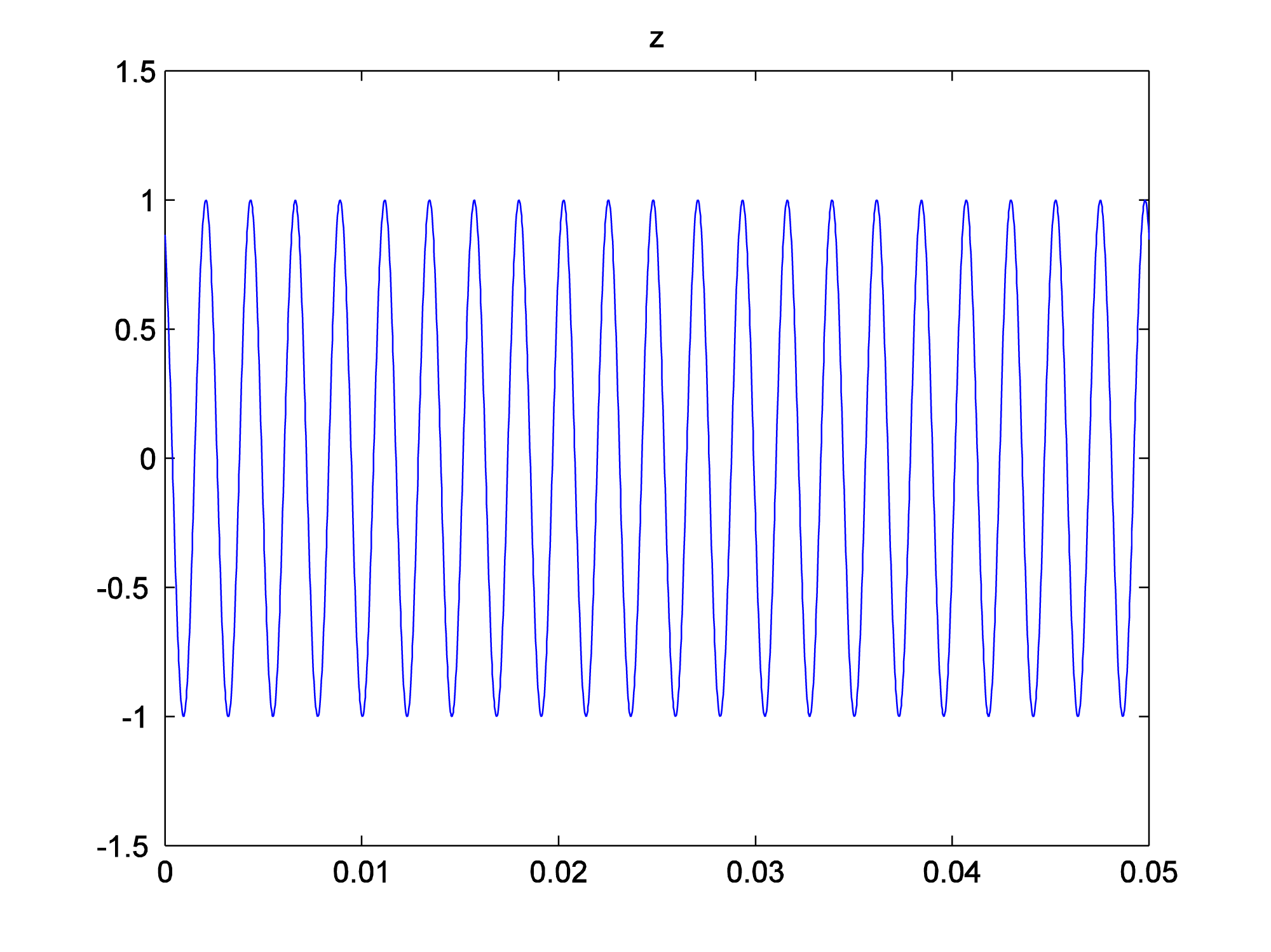
plot(t,z);
axis([0 0.05 -1.5 1.5]);
title('z');

We look at only the first 0.05 seconds of the waveforms in order to see their shape better. You can see the phase shifts in the figures below. The second and third waves don’t start at 0 on the vertical axis.

Now we add the three sine waves to create a composite wave that has three frequency components at three different phases.

a = (x + y + z)/3;

Notice that we divide the summed sound waves by three so that the sound doesn’t clip. You can graph the three-component sound wave with the following:

figure;
plot(t, a);
axis([0 0.05 -1.5 1.5]);
title('a = x + y + z');

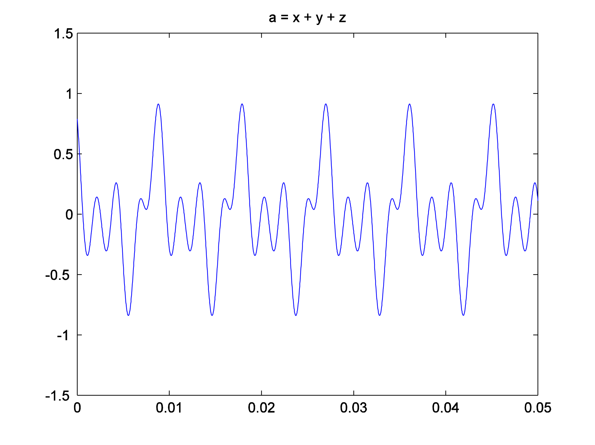
This is a graph of the sound wave in the time domain. You could call it an impulse response graph, although when you’re looking at a sound file like this, you usually just think of it as “sound data in the time domain.” The term “impulse response” is used more commonly for time domain filters, as we’ll see in Chapter 7. You might want to play the sound to be sure you have what you think you have. The sound function requires that you tell it the number of samples it should play per second, which for our simulation is 44,100.

sound(a, sr);

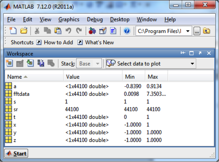
When you play the sound file and listen carefully, you can hear that it has three tones. MATLAB’s Fourier transform (fft) returns an array of double complex values (double-precision complex numbers) that represent the magnitudes and phases of the frequency components.

fftdata = fft(a);

In MATLAB’s workspace window, fftdata values are labeled as type double, giving the impression that they are real numbers, but this is not the case. In fact, the Fourier transform produces complex numbers, which you can verify by trying to plot them in MATLAB. The magnitudes of the complex numbers are given in the Min and Max fields, which is computed by the abs function. For a complex number $$a+bi$$, the magnitude is computed as $$\sqrt{a^{2}+b^{2}}$$. MATLAB does this computation and yields the magnitude.

To plot the results of the fft function such that the values represent the magnitudes of the frequency components, we first apply the abs function to fftdata.

fftmag = abs(fftdata);

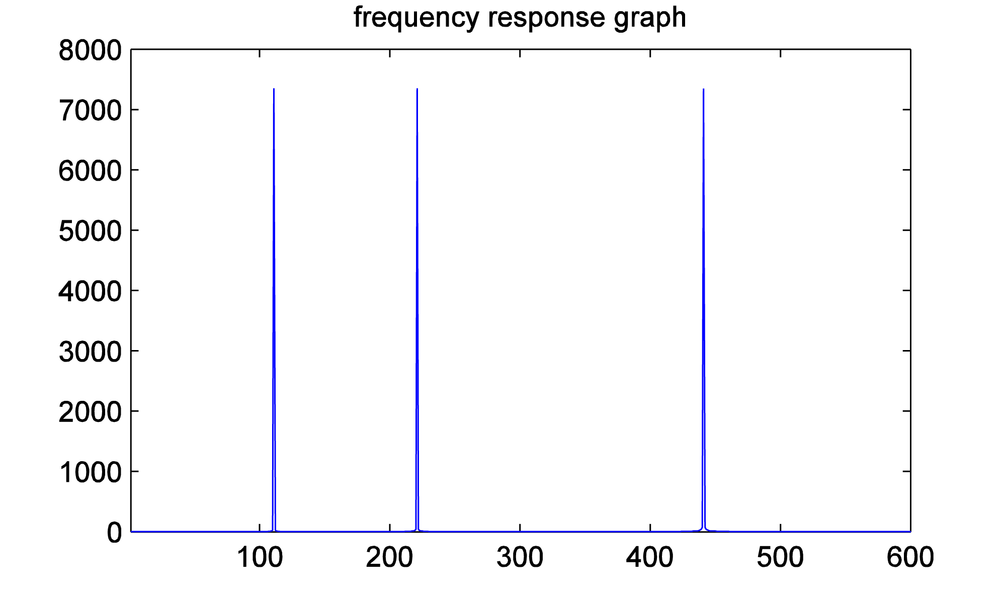
Let’s plot the frequency components to be sure we have what we think we have. For a sampling rate of sr on an array of sample values of size N, the Fourier transform returns the magnitudes of $$N/2$$ frequency components evenly spaced between 0 and sr/2 Hz. (We’ll explain this completely in Chapter 5.)   Thus, we want to display frequencies between 0 and sr/2 on the horizontal axis, and only the first sr/2 values from the fftmag vector.

figure;
freqs = [0: (sr/2)-1];
plot(freqs, fftmag(1:sr/2));

[aside]If we would zoom in more closely at each of these spikes at frequencies 110, 220, and 440 Hz, we would see that they are not perfectly horizontal lines.  The “imperfect” results of the FFT will be discussed later in the sections on FFT windows and windowing functions.[/aside] When you do this, you’ll see that all the frequency components are way over on the left side of the graph. Since we know our frequency components should be 110 Hz, 220 Hz, and 440 Hz, we might as well look at only the first, say, 600 frequency components so that we can see the results better. One way to zoom in on the frequency response graph is to use the zoom tool in the graph window, or you can reset the axis properties in the command window, as follows.

axis([0 600 0 8000]);

This yields the frequency response graph for our composite wave, which shows the three frequency components.

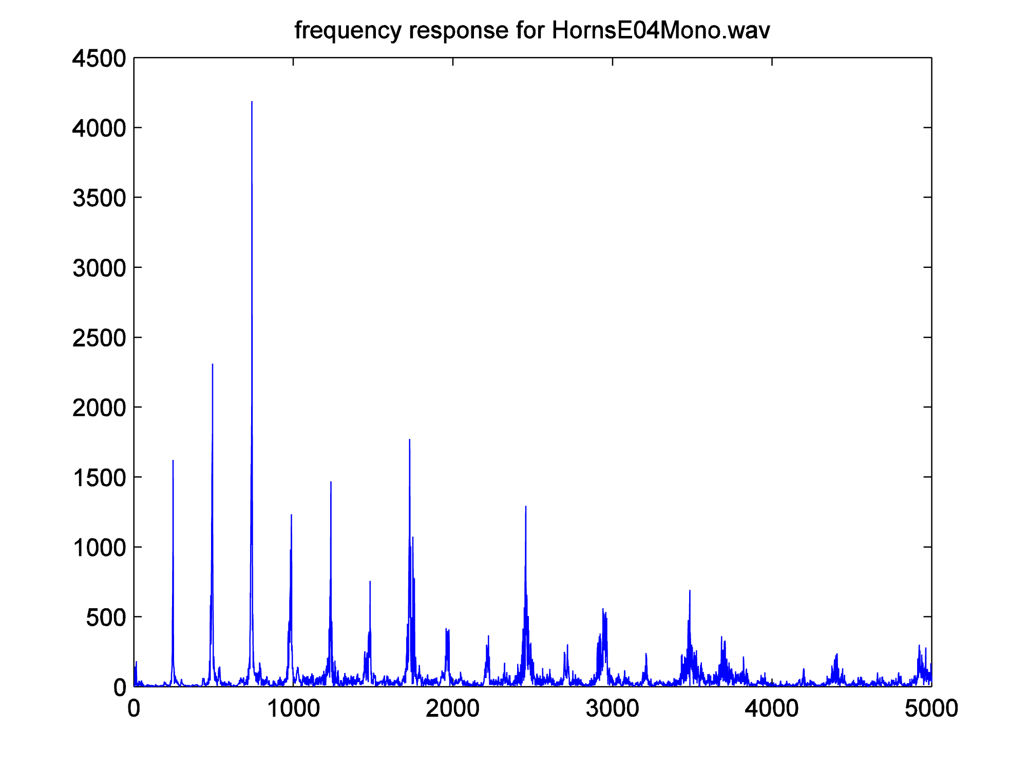
To get the phase response graph, we need to extract the phase information from the fftdata. This is done with the angle function. We leave that as an exercise. Let’s try the Fourier transform on a more complex sound wave – a sound file that we read in.

y = audioread('HornsE04Mono.wav');

As before, you can get the Fourier transform with the fft function.

fftdata = fft(y);

You can then get the magnitudes of the frequency components and generate a frequency response graph from this.

fftmag = abs(fftdata);
figure;
freqs = [0:(sr/2)-1];
plot(freqs, fftmag(1:sr/2));
axis([0 sr/2 0 4500]);
title('frequency response for HornsE04Mono.wav'); 

Let’s zoom in on frequencies up to 5000 Hz.

axis([0 5000 0 4500]);

The graph below is generated.

The inverse Fourier transform gives us back our original sound data in the time domain.

ynew = ifft(fftdata);

If you compare y with ynew, you’ll see that the inverse Fourier transform has recaptured the original sound data.

When we applied the Fourier transform in MATLAB in Section 2.3.9, we didn’t specify a window size.  Thus, we were applying the FFT to the entire piece of audio. If you listen to the WAV file HornsE04Mono.wav, a three second clip, you’ll first hear some low tubas and them some higher trumpets. Our graph of the FFT shows frequency components up to and beyond 5000 Hz, which reflects the sounds in the three seconds. What if we do the FFT on just the first second (44100 samples) of this WAV file, as follows? The resulting frequency components are shown in Figure 2.49.

y = audioread('HornsE04Mono.wav');
sr = 44100;
freqs = [0:(sr/2)-1];
ybegin = y(1:44100);
fftdata2 = fft(ybegin);
fftdata2 = fftdata2(1:22050);
plot(freqs, abs(fftdata2));
axis([0 5000 0 4500]);

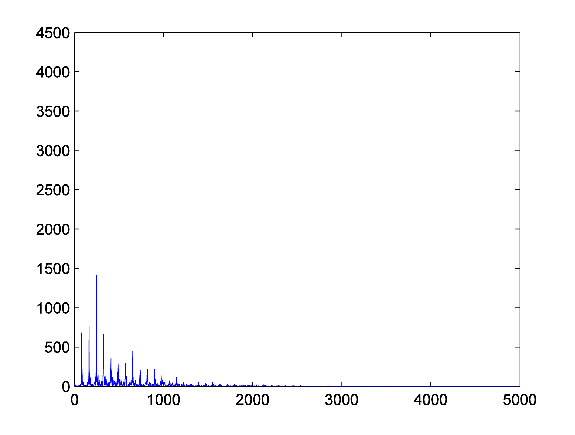
What we’ve done is focus on one short window of time in applying the FFT. An FFT window is a contiguous segment of audio samples on which the transform is applied. If you consider the nature of sound and music, you’ll understand why applying the transform to relatively small windows makes sense. In many of our examples in this book, we generate segments of sound that consist of one or more frequency components that do not change over time, like a single pitch note or a single chord being played without change. These sounds are good for experimenting with the mathematics of digital audio, but they aren’t representative of the music or sounds in our environment, in which the frequencies change constantly. The WAV file HornsE04Mono.wav serves as a good example. The clip is only three seconds long, but the first second is very different in frequencies (the pitches of tubas) from the last two seconds (the pitches of trumpets). When we do the FFT on the entire three seconds, we get a kind of “blurred” view of the frequency components, because the music actually changes over the three second period. It makes more sense to look at small segments of time. This is the purpose of the FFT window.

Figure 2.50 shows an example of how FFT window sizes are used in audio processing programs. Notice the drop down menu, which gives you a choice of FFT sizes ranging from 32 to 65536 samples. The FFT window size is typically a power of 2. If your sampling rate is 44,100 samples per second, then a window size of 32 samples is about 0.0007 s, and a window size of 65536 is about 1.486 s.

There’s a tradeoff in the choice of window size. A small window focuses on the frequencies present in the sound over a short period of time. However, as mentioned earlier, the number of frequency components yielded by an FFT of size N is N/2. Thus, for a window size of, say, 128, only 64 frequency bands are output, these bands spread over the frequencies from 0 Hz to sr/2 Hz where sr is the sampling rate. (See Chapter 5.) For a window size of 65536, 37768 frequency bands are output, which seems like a good thing, except that with the large window size, the FFT is not isolating a short moment of time. A window size of around 2048 usually gives good results. If you set the size to 2048 and play the piece of music loaded into Audition, you’ll see the frequencies in the frequency analysis view bounce up and down, reflecting the changing frequencies in the music as time pass.

Even if you’re not a musician, if you plan to work in the realm of digital sound you’ll benefit from an understanding of the basic concepts and vocabulary of music. The purpose of this chapter is to give you this foundation.

This chapter describes the vocabulary and musical notation of the Western music tradition – the music tradition that began with classical composers like Bach, Mozart, and Beethoven and that continues as the historical and theoretic foundation of music in the United States, Europe, and Western culture. The major and minor scales and chords are taken from this context, which we refer to as Western music. Many other types of note progressions and intervals have been used in other cultures and time periods, leading to quite different characteristic sounds: the modes of ancient Greece, the Gregorian chants of the Middle Ages, the pentatonic scale of ancient Oriental music, the Hindu 22 note octave, or the whole tone scale of Debussy, for example. While we won’t cover these, we encourage the reader to explore these other musical traditions.

To give us a common language for understanding music, we focus our discussion on the musical notation used for keyboards like the piano. Keyboard music expressed and notated in the Western tradition provides a good basic knowledge of music and gives us a common vocabulary when we start working with MIDI in Chapter 6.

Musicians learn to sing, play instruments, and compose music using a symbolic language of music notation. Before we can approach this symbolic notation, we need to establish a basic vocabulary.

In the vocabulary of music, a sound with a single fundamental frequency is called a tone. The fundamental frequency of a tone is the frequency that gives the tone its essential pitch. The piccolo plays tones with higher fundamental frequencies than the frequencies of a flute, and thus it is higher pitched.

A tone that has an onset and a duration is called a note. The onset of the note is the moment when it begins. The duration is the length of time that the note remains audible. Notes can be represented symbolically in musical notation, as we’ll see in the next section. We will also use the word “note” interchangeably with “key” when referring to a key on a keyboard and the sound it makes when struck.

As described in Chapter 2, tones created by musical instruments, including the human voice, are not single-frequency. These tones have overtones at frequencies higher than the fundamental. The overtones create a timbre, which distinguishes the quality of the tone of one instrument or singer from another. Overtones add a special quality to the sound, but they don’t change our overall perception of the pitch. When the frequency of an overtone is an integer multiple of the fundamental frequency, it is a harmonic overtone. Stated mathematically for frequencies $$f_{1}$$ and $$f_{2}$$, if $$f_{2}=nf_{1}$$ and n is a positive integer, then $$f_{2}$$ is a harmonic frequency relative to fundamental frequency $$f_{1}$$. Notice that every frequency is a harmonic frequency relative to itself. It is called the first harmonic, since $$n=1$$. The second harmonic is the frequency where $$n=2$$. For example, the second harmonic of 440 Hz is 880 Hz; the third harmonic of 440 Hz is 3*440 Hz = 1320 Hz; the fourth harmonic of 440 Hz is 4*440 Hz = 1760 Hz; and so forth. Musical instruments like pianos and violins have harmonic overtones. Drums beats and other non-pitched sounds have overtones that are not harmonic.

Another special relationship among frequencies is the octave. For frequencies $$f_{1}$$ and $$f_{2}$$, if $$f_{2}=2^{n}f_{1}$$ where n is a positive integer, then $$f_{1}$$ and $$f_{2}$$ “sound the same,” except that $$f_{2}$$ is higher pitched than $$f_{1}$$. Frequencies $$f_{1}$$ and $$f_{2}$$ and are separated by n octaves. Another way to describe the octave relationship is to say that each time a frequency is moved up an octave, it is multiplied by 2. A frequency of 880 Hz is one octave above 440 Hz; 1760 Hz is two octaves above 440 Hz; 3520 Hz is three octaves above 440 Hz; and so forth. Two notes separated by one or more octaves are considered equivalent in that one can replace the other in a musical composition without disturbing the harmony of the composition.

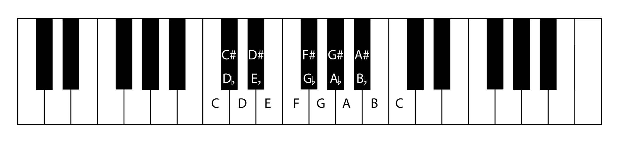
In Western music, an octave is separated into 12 frequencies corresponding to notes on a piano keyboard, named as shown in Figure 3.1. From C to B we have 12 notes, and then the next octave starts with another C, after which the sequence of letters repeats. An octave can start on any letter, as long as it ends on the same letter. (The sequence of notes is called an octave because there are eight notes in a diatonic scale, as is explained below.) The white keys are labeled with the letters. Each of the black keys can be called by one of two names. If it is named relative to the white key to its left, a sharp symbol is added to the name, denoted C#, for example. If it is named relative to the white key to its right, a flat symbol is added to the name, denoted D♭, for example.

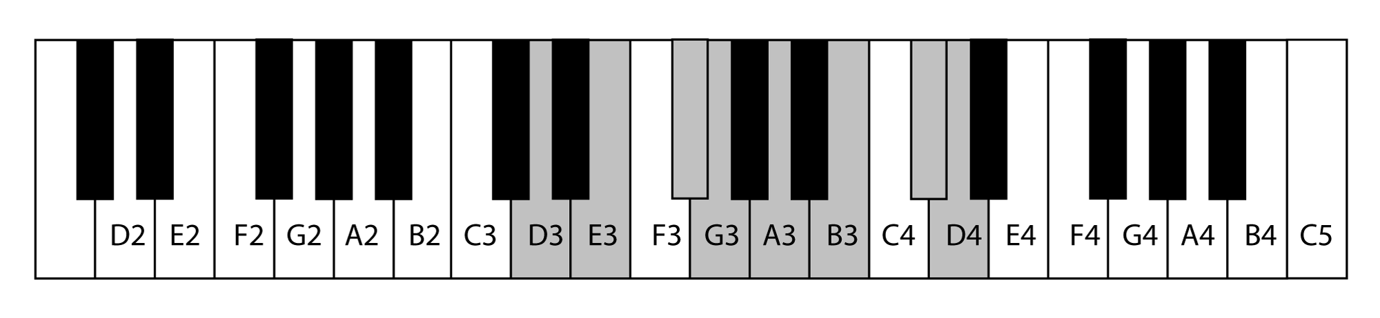
Each note on a piano keyboard corresponds to a physical key that can be played. There are 88 keys on a standard piano keyboard. MIDI keyboards are usually smaller. Since the notes from A through G are repeated on the keyboard, they are sometimes named by the number of the octave that they’re in, as shown in Figure 3.2.

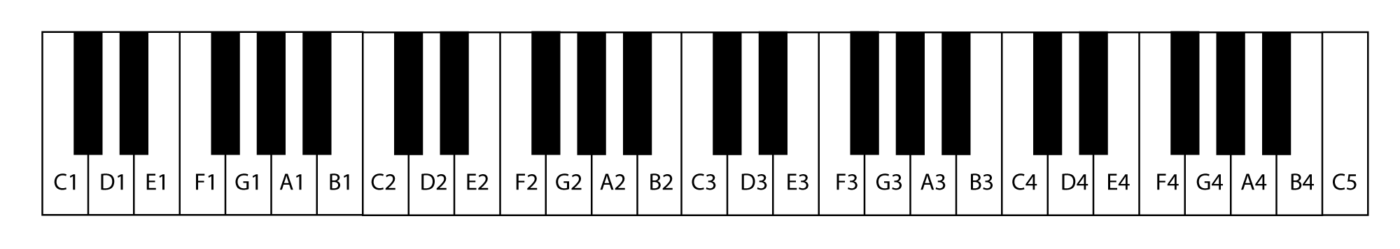
Middle C on a standard piano has a frequency of approximately 262 Hz. On a piano with 88 keys, middle C is the fourth C, so it is called C4. On the smaller MIDI keyboard shown above, it is C3. Middle C is the central position for playing the piano, with regard to where the right and left hands of the pianist are placed. The standard reference point for tuning a piano is the A above middle C, which has a frequency of 440 Hz. This means that the next A going up the keys to the right has a frequency of 880 Hz. A note of 880 Hz is one octave away from 440 Hz, and both are called A on a piano keyboard.

The interval between two consecutive keys (also called notes) on a keyboard, whether the keys are black or white, is called a semitone. A semitone is the smallest frequency distance between any two notes. Neighboring notes on a piano keyboard (and equivalently, two neighboring notes on a chromatic scale) are separated by a frequency factor of approximately 1.05946. This relationship is described more precisely in the equation below.

[equation caption=”Equation 3.1″]

Let f be the frequency of a note k. Then the note one octave above f has a frequency of $$2f$$. Given this octave relationship and the fact that there are 12 notes in an octave, the frequency of the note after k on a chromatic scale is $$\sqrt[12]{2}\, f\approx 1.05946\, f$$.

[/equation]

Thus, the factor 1.05946 defines a semitone. If two notes are divided by a semitone, then the frequency of the second is 1.05946 times the frequency of the first. The other frequencies between semitones are not used in Western music (except in pitch bending).

Two semitones constitute a whole tone, as illustrated in Figure 3.3. Semitones and whole tones can also be called half steps and whole steps (or just steps), respectively. They are illustrated in Figure 3.3.

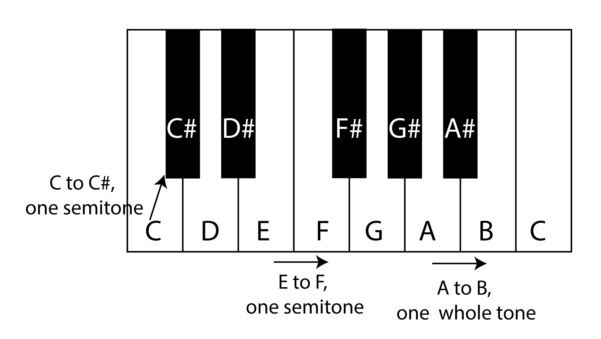
The symbol #, called a sharp, denotes that a note is to be raised by a semitone. When you look at the keyboard in Figure 3.3, you can see that moving up by a semitone takes you to the F key. Thus E# denotes and sounds the same note as F. When two notes have different names but are the same pitch, they said to be enharmonically equivalent.

The symbol♭, called a flat, denotes that a note is to be lowered by a semitone. C♭is enharmonically equivalent to B. A natural symbol ♮removes a sharp or flat from a note when it follows the same note in a measure. Sharps, flats, and naturals are examples of accidentals, symbols that raise or lower a note by a semitone.

It’s fascinating to consider the way humans perceive sound, experiencing some sounds as musical and some as noise. Understanding frequency components and harmonics gives us some insight into why music is pleasing to our senses.

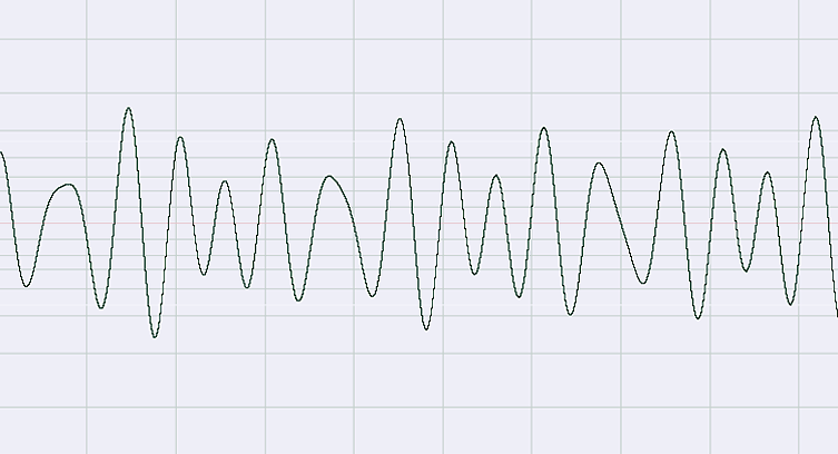
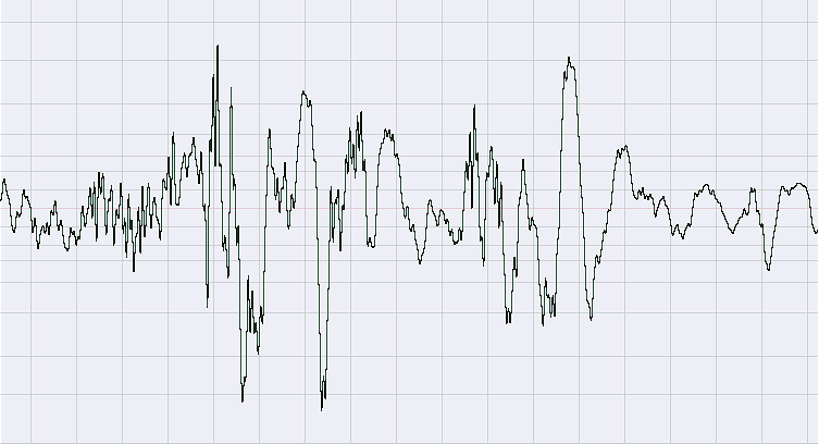
Consider the waveforms in Figure 3.4 and Figure 3.5. The first shows the notes C, E, and G played simultaneously. The second is a recording of scratching sounds. The first waveform has a regular pattern because the frequency components are pure sine waves with a harmonic relationship. Patterns such as this are common in music and the sounds produced by acoustic instruments. The second sound has no pattern; the relationship of the frequency components is random at any moment in time and varies randomly over time. Randomness is characteristic of noise.

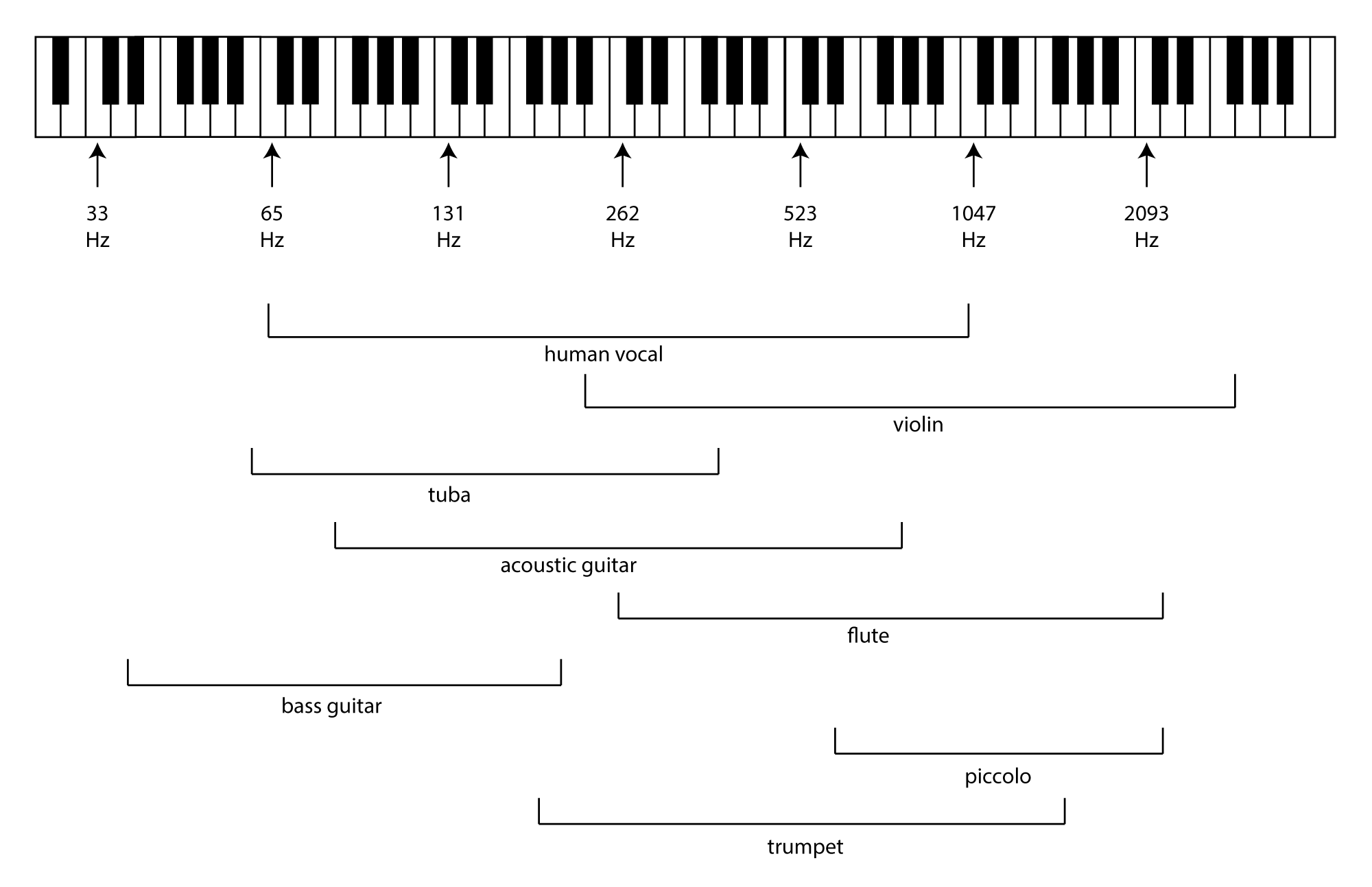
Musical instruments like violins, pianos, clarinets, and flutes naturally emit sounds with unique harmonic components. Each instrument has an identifiable timbre governed by these harmonic components. This timbre is sometimes called the instrument’s tone color, which results from its shape, the material of which it is made, its resonant structure, and the way it is played. These physical properties result in the instrument having a characteristic range of frequencies and harmonics. (See Figure 3.6.)

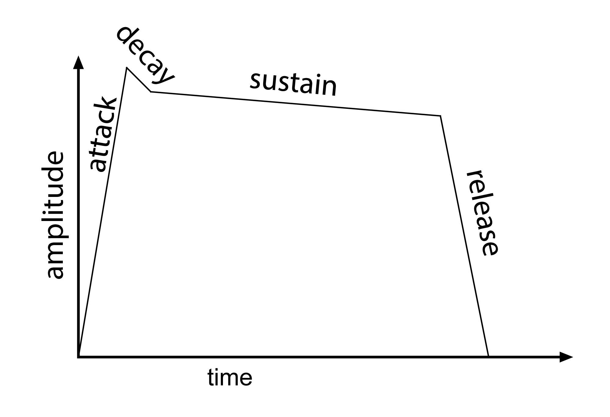
Instruments also are distinguished by the amplitude envelope for individual sounds created by the instrument. The amplitude envelope gives a sense of how the loudness of a single note changes over the short period of time when it is played. When you play a certain instrument, do you burst into the note or slide into it gently? Does the note linger or end abruptly? Imagine a single note played by a flute compared to the same note played by a piano. Although you don’t always play a piano note the same way – for example, you can strike the key gently or briskly – it’s still possible to get a picture of a typical amplitude envelope for each instrument and see how they differ. The amplitude envelope consists of four components: attack, decay, sustain, and release, abbreviated ADSR, as illustrated in Figure 3.7. The attack is the time between when the sound is first audible and when it reaches its maximum loudness. The decay is the period of time when the amplitude decreases. Then the amplitude can level to a plateau in the sustain period. The release is when the sound dies away. The attack of a trumpet is relatively sudden, rising steeply to its maximum, because you have to blow pretty hard into a trumpet before the sound starts to come out. With a violin, on the other hand, you can stroke the bow across a string gently, creating a longer, less steep attack. The sustain of the violin note might be longer than that of the trumpet, also, as the bow continues to stroke across the string. Of course, these envelopes vary in individual performances depending on the nature of the music being played. Being aware of the amplitude envelope that is natural to an instrument helps in the synthesis of music. Tools exist for manipulating the envelopes of MIDI samples so that they sound more realistic or convey the spirit of the music better, as we’ll see in Chapter 6.

The combination of harmonic instruments in an orchestra gives rise to an amazingly complex pattern of frequencies that, taken together, express the aesthetic intent of the composer. Non-harmonic instruments – e.g., percussion instruments – can contribute to beauty or harshness of the aesthetic intent. Drums, gongs, cymbals, and maracas are not musical in the same sense that flutes and violins are. The partials (frequency components) emitted by percussion instruments are not integer multiples of a fundamental, and thus these instruments don’t have a distinct pitch with harmonic overtones. However, percussion instruments contribute accents to music, called transients. Transients are high-frequency sounds that come in short bursts. Their attacks are quite sharp, their sustains are short, and their releases are steep. These percussive sounds are called “transient” because they come and go quickly. Because of this, we have to be careful not to edit them out with noise gates and other processors that react to sudden changes of amplitude. Even with their non-harmonic nature, transients add flavor to an overall musical performance, and we wouldn’t want to do without them.

Let’s return now to a bit more music theory as we establish a working vocabulary and an understanding of musical notation.

[wpfilebase tag=file id=32 tpl=supplement /]

A scale is an ordered set of musical notes that are defined relative to a fundamental frequency, also known as the tonal center or tonic. There are different types of scales defined in music, which vary in the number of notes played and the intervals between the notes.

Table 3.1 lists seven types of scales divided into three general categories – chromatic, diatonic, and pentatonic. A list of 1s and 2s is a convenient way to represent the semitone intervals between each note in a scale. Moving by a semitone is represented by the number 1, meaning “move over a semitone from the previous note.” Moving by a whole tone is represented by the number 2, meaning “move over two semitones from the previous note.”

A chromatic scale consists of 12 notes. (However, when the scale is played, usually the 13th note is played, which is one octave above the first note. This note is note counted as one in the scale because it is the same note as the first one, but one octave above.)  A chromatic scale starts on any pitch, and then each note is separated from the previous one by a semitone. Thus the pattern of a chromatic scale (where the 13th note is played) is represented simply by the list [1 1 1 1 1 1 1 1 1 1 1 1]. Note that while 13 notes are played, there are only 12 numbers on the list. The first note is played, and then the list represents how many semitones to move over to play the following notes.

A diatonic scale has seven notes. In a major diatonic scale, the pattern is [2 2 1 2 2 2 1], assuming again that one more note is added as the scale is played, ending the scale one octave above where it began. This means, “start on the first note, move over by a tone, a tone, a semitone, a tone, a tone, a tone, and a semitone.” A major diatonic scale beginning on D3 (and adding an extra note) is depicted in Figure 3.8. Those who grow up in the tradition of Western music become accustomed to the sequence of sounds in a diatonic scale as the familiar “do re mi fa so la ti do.” A diatonic scale can start on any note, but all diatonic scales have the same pattern of sound in them; one scale is just higher or lower than another. Diatonic scales sound the same because the differences in the frequencies between consecutive notes on the scale follow the same pattern, regardless of the note you start on.

A minor diatonic scale is played in the pattern [2 1 2 2 1 2 2]. This pattern is also referred to as the natural minor. There are variations of minor scales as well. The harmonic minor scale follows the pattern [2 1 2 2 1 3 1], where 3 indicates a step and a half. The melodic minor follows the pattern [2 1 2 2 2 2 1] in the ascending scale, and [2 2 1 2 2 1 2] in the descending scale (played from highest to lowest note). The pattern of whole and half steps for major and minor scales are given in Table 3.1.

[table caption=”Table 3.1 Pattern of whole and half steps for various scales” width=”80%” colalign=”center|center”]

Type of scale,Pattern of whole steps (2) and half steps (1)

chromatic,1 1 1 1 1 1 1 1 1 1 1

major diatonic,2 2 1 2 2 2 1

natural minor diatonic,2 1 2 2 1 2 2

harmonic minor diatonic,2 1 2 2 1 3 1

melodic minor diatonic,2 1 2 2 2 2 1 ascending~~2 2 1 2 2 1 2 descending

pentatonic major,2 3 2 2 3 or 2 2 3 2 3

pentatonic minor,3 2 3 2 2 or 3 2 2 3 2

[/table]

Two final scale types ought to be mentioned because of their prevalence in music of many different cultures. These are the pentatonic scales, created from just five notes. An example of a pentatonic major scale results from playing only black notes beginning with F#. This is the interval pattern 2 2 3 2 3, which yields the scale F#, G#, A#, C#, D#, F#. If you play these notes, you might recognize them as the opening strain from “My Girl” by the Temptations, a pop song from the 1960s. Another variant of the pentatonic scale has the interval pattern 2 3 2 2 3, as in the notes C D F G A C. These notes are the ones used in the song “Ol’ Man River” from the musical Showboat (Figure 3.9).

[table caption=”Figure 3.9 Pentatonic scale used in “Ol Man River”” th=”0″ width=”250px”]

“Ol’ man river,”
C   C     D F

Dat ol’ man river

D   C   C     D F
He mus’know sumpin’

G   A       A       G   F
“But don’t say nuthin’,”

G     A   C     D   C
He jes’keeps rollin’

D   C   C         A   G
He keeps on rollin’ along.

A   C     C     A   G   A F

[/table]

To create a minor pentatonic scale from a major one, begin three semitones lower than the major scale and play the same notes. Thus, the pentatonic minor scale relative to F#, G#, A#, C#, D#, F# would be D#, F#, G#, A#, C#, D#, which is a D# pentatonic minor scale. The minor relative to C D F G A C would be A C D F G A, which is an A pentatonic minor scale. As with diatonic scales, pentatonic scales can be set in different keys.

It’s significant that a chromatic scale really has no variation in the sequence of notes played. We simply move up by semitone steps of [1 1 1 1 1 1 1 1 1 1 1 1 1]. The distance between neighboring notes is always the same. In a diatonic scale, on the other hand, there is a pattern of varying half steps and whole steps between notes. The pattern gives notes different importance to the ear relative to the key, also called the tonic. This difference in the roles that notes play in a diatonic scale is captured in the names given to these notes, listed in Table 3.2. Roman numerals are conventionally used for the positions of these notes.   These names will become more significant when we discuss chords later in this chapter.

[table caption=”Table 3.2 Technical names for notes on a diatonic scale” width=”250px” colalign=”center|center”]

Position,Name for note

I,tonic

II,supertonic

III,mediant

IV,subdominant

V,dominant

VI,submediant

VII,leading note

[/table]

3.1.5.1 Score

In the tradition of Western music, a system of symbols has been devised to communicate and preserve musical compositions. This system includes symbols for notes, timing, amplitude, and keys. A musical composition is notated on a score. There are scores of different types, depending on the instrument being played. The score we describe is for a standard piano, MIDI controller or keyboard score.

A piano score consists of two staves, each of which consists of five horizontal lines. The staves are drawn one above the other. The top staff is called the treble clef, representing the notes that are played by the right hand. The symbol for the treble clef is placed at the far left of the top staff. (The word “clef” is French for “key.”) The bottom staff is the bass clef, representing what is played with the left hand. The symbol for the bass clef is placed at the far left of the bottom staff. A blank score with no notes on it is pictured in Figure 3.10.

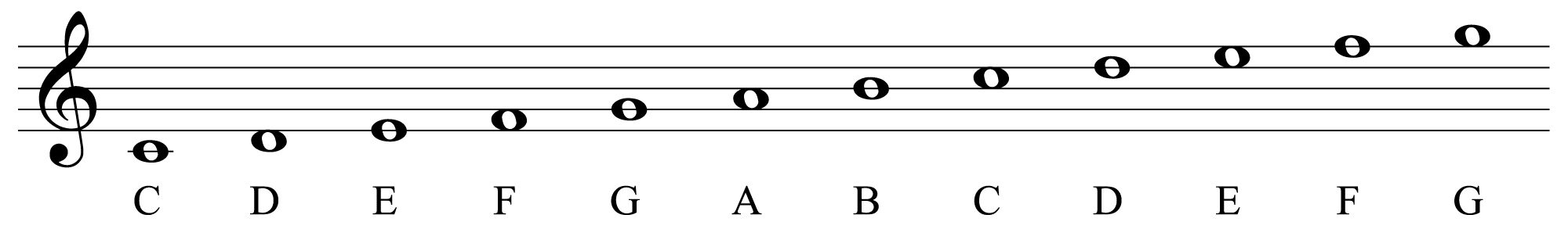
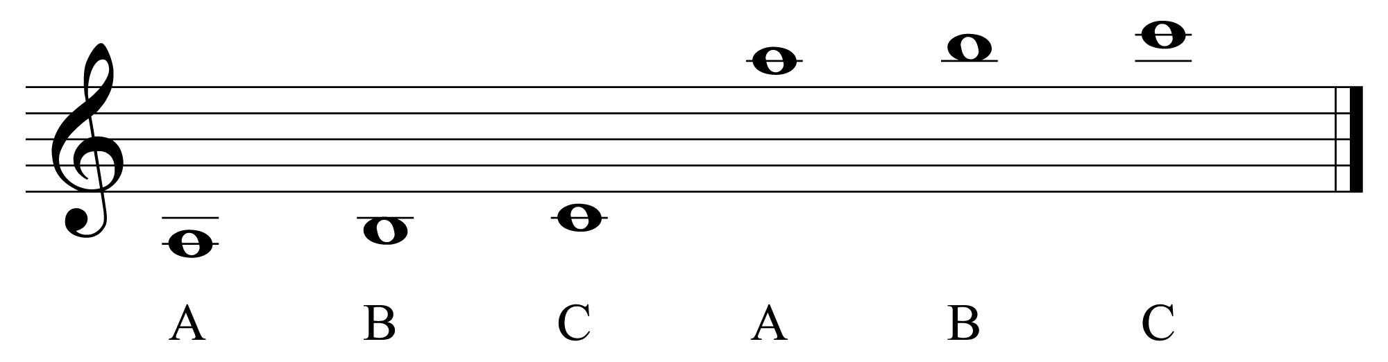
Each line and space on the treble and bass clef staves corresponds to a note on the keyboard to be played, as shown in Figure 3.11 and Figure 3.12. A whole note (defined below) is indicated by an oval like those shown. The letter for the corresponding note is given in the figures. The letters are ordinarily not shown on a musical score. We have them here for information only. The treble clef is sometimes called the G clef because its bottom portion curls around the line on the staff corresponding to the note G. The bass clef is sometimes called the F clef because it curls around the line on the staff corresponding to the note F.

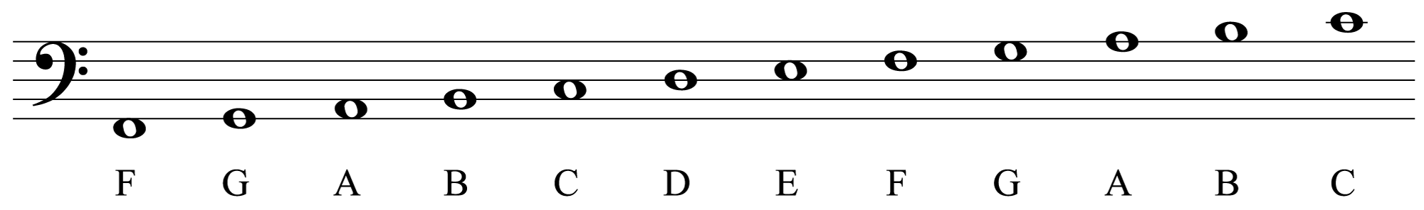
It’s possible to place a note below or above one of the staves. The note’s distance from the staff indicates what note it is. If it’s a note that would fall on a line, a small line is placed through it, and if the note would fall on a space, a line is placed under or over it. The lines between the staff and the upper or lower note are displayed by a short line, also. The short lines that are used to extend the staff are called ledger lines. Examples of notes with ledger lines are shown in Figure 3.13 and Figure 3.14.

[wpfilebase tag=file id=33 tpl=supplement /]

Beginners who are learning to read music often use mnemonics to remember the notes corresponding to lines and spaces on a staff. For example, the lines on the treble clef staff, in ascending order, correspond to the notes E, G, B, D, and F, which can be memorized with the mnemonic “every good boy does fine.” The spaces on the treble clef staff, in ascending order, spell the word FACE. On the bass clef, the notes G, B, D, F, and A can be remembered as “good boys deserve favor always,” and the spaces A, C, E, G can be remembered as “a cow eats grass” (or whatever mnemonics you like).

3.1.5.2 Notes and their Durations

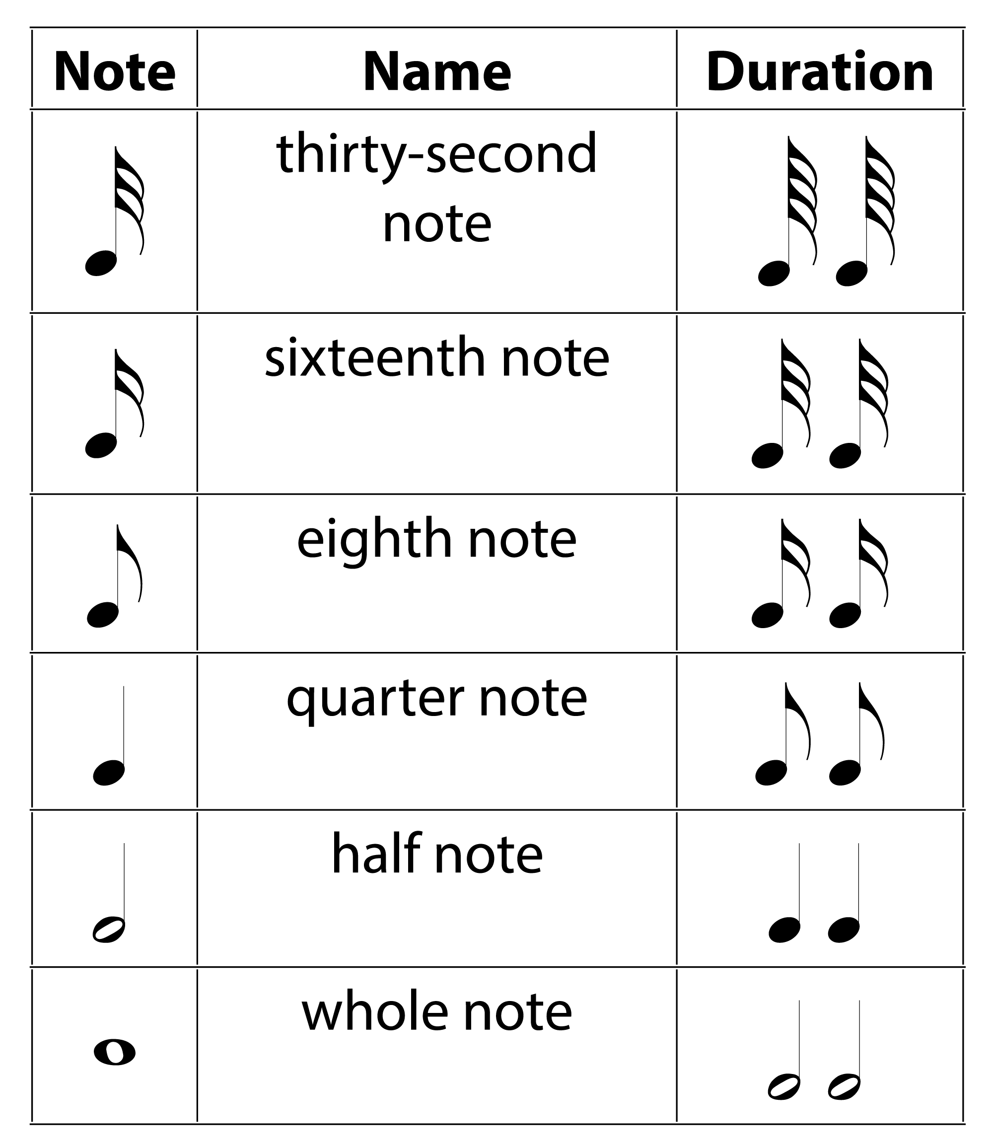
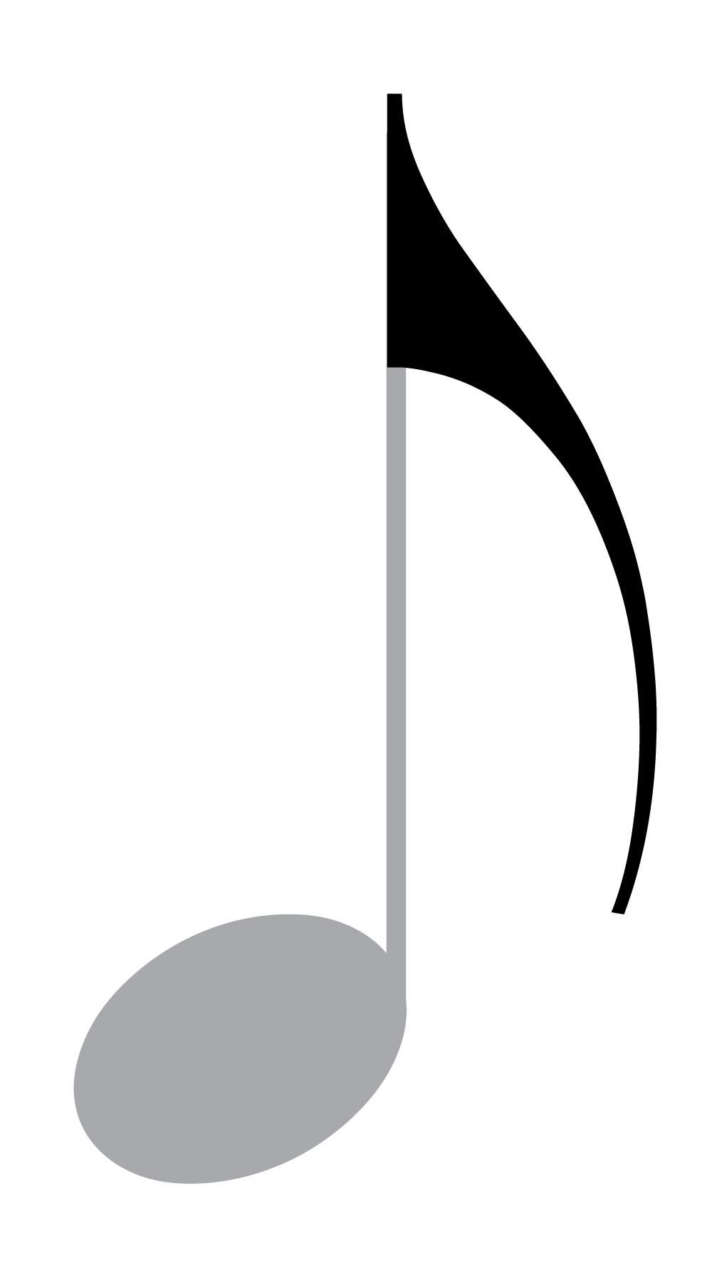
There are types of notes – whole notes, half notes, quarter notes, and so forth, as shown in Table 3.3. On the score, you can tell what type a note is by its shape and whether or not the note is filled in (black or white). The durations of notes are defined relative to each other, as you can see in the table. We could continue to create smaller and smaller notes, beyond those listed in the table, by adding more flags to a note. The part of the note called the flag is shown in Figure 3.15. Each time we add a flag, we divide the duration of the previously defined note by 2.

3.1.5.3 Rhythm, Tempo, and Meter

[wpfilebase tag=file id=109 tpl=supplement /]

The timing of a musical composition and its performance is a matter of meter, tempo, and rhythm.

Meter is the regular grouping of beats and placement of accents in notes. Since the duration of different notes are defined relative to each other, we have to have a baseline. This is given in a score’s time signature (a synonym of meter), which indicates which type of note gets one beat (quarter note, eighth note, etc.). (There are two types of meter – simple and compound. We are considering only simple meter here.)

Beats and notes are grouped into measures. Measures are sometimes called bars because they are separated from each other on the staff by a vertical line called a bar line.

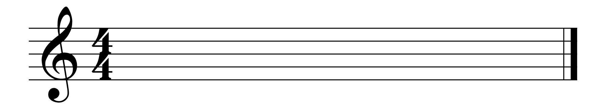
A time signature of $$\frac{x}{y}$$, where x and y are integers, indicates that there are x beats to a measure, and a note of size $$\frac{1}{y}$$gets one beat. (A half note is size ½, a quarter note is size ¼, and so forth.) A time signature of $$\frac{4}{4}$$ time is shown in Figure 3.16, indicating four beats to a measure with a quarter note getting one beat. A time signature of $$\frac{3}{4}$$ indicates three beats to a measure with a quarter note getting one beat. $$\frac{3}{4}$$ is the meter for a waltz.

If the time signature of a piece is $$\frac{4}{4}$$, then there are four beats to a measure and each quarter note gets a beat. Consider the score in Figure 3.17, which shows you how to play “Twinkle, Twinkle Little Star” in $$\frac{4}{4}$$time in the key of C. Each of the six syllables in “Twin-kle Twin-kle Lit-tle” corresponds to a quarter note, and each is given equal time – one beat – in the first measure. Then the note corresponding to the word “star” is held for two beats in the second measure. Measures three and four are similar to measures one and two.

Tempo is the pace at which music is performed. We can sing “Yankee Doodle” in a fast, snappy pace or slowly, like a dirge. Obviously, most songs have tempos that seem more appropriate for them.

The tempo of a musical piece depends on which type of note is given one beat and how many beats there are per second. Tempo can be expressed at the beginning of the score explicitly, in terms of beats per minute (BPM). For example, a marking such as bpm = 72, ♩ = 72, or mm = 72 (for Maezel’s metronome) placed above a measure indicates that a tempo of 72 beats per minute is recommend from this point on, with a quarter note getting one beat. Alternatively, an Italian key word like allegro or andante can be used to indicate the beats per minute in a way that can be interpreted more subjectively. A list of some of these tempo markings is given in Table 3.4.

[table caption=”Table 3.4″ width=”80%” colalign=”center|center”]

Tempo Marking,Meaning

prestissimo,extremely fast (more than 200 BPM)

presto,very fast (168 – 200 BPM)

allegro,fast (120 – 168 BPM)

moderato,moderately (108 – 120 BPM)

andante,“at a walking pace” (76 – 108 BPM)

adagio,slowly (66 – 76 BPM)

lento or largo,very slowly (40 – 60 BPM)

[/table]

Students learning to play the piano sometimes use a device called a metronome to tick out the beats per minute while they practice (also known as a click).   Metronomes are also usually built into MIDI sequencers and keyboards.

The Google dictionary gives three definitions of rhythm:  

1. a strong, regular, repeated pattern of movement or sound; 
2. the systematic arrangement of musical sounds, principally according to duration and periodic stress; and 
3. a particular type of pattern formed by rhythm. 

You can see from these definitions that rhythm generally is based on the arrangement of notes of different durations that are sounded over time. Rhythm also includes the accenting of notes, which generally has a pattern. An example of this aspect of rhythm is illustrated by the rhythm of the message SOS in Morse code.

Rhythm and meter are interrelated. Meter is the macro-pattern of beats and accents that remains consistent throughout the song. Rhythm is the micro-pattern that gives the song its individuality. Once the meter is set for a section of a musical composition, the number of beats per measure must fit within that time signature. However, which particular types of rests and  notes — whole, half, quarter, eighth, etc. —  are chosen to add up to the number of beats per measure is up to the composer.

Rhythm is a complicated feature of music and is difficult to define in a general sense because of its many variations, so we won’t go into detail about it here.

3.1.5.4 Rests and their Durations

[wpfilebase tag=file id=138 tpl=supplement /]

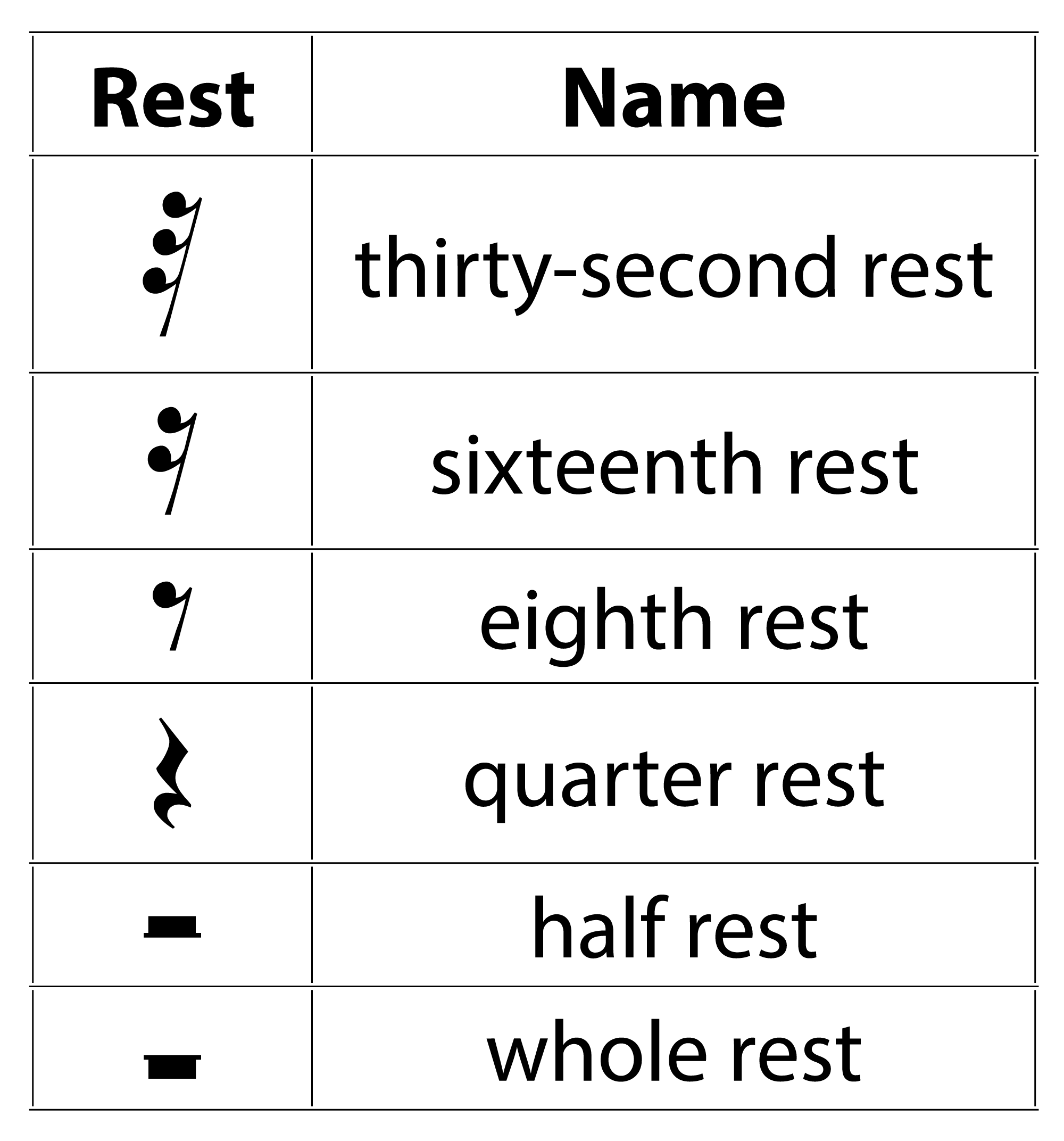
The duration of silence between notes is indicated by a rest. The symbols for rests are given in Table 3.5. The length of a rest corresponds to the length of a note of the same name.

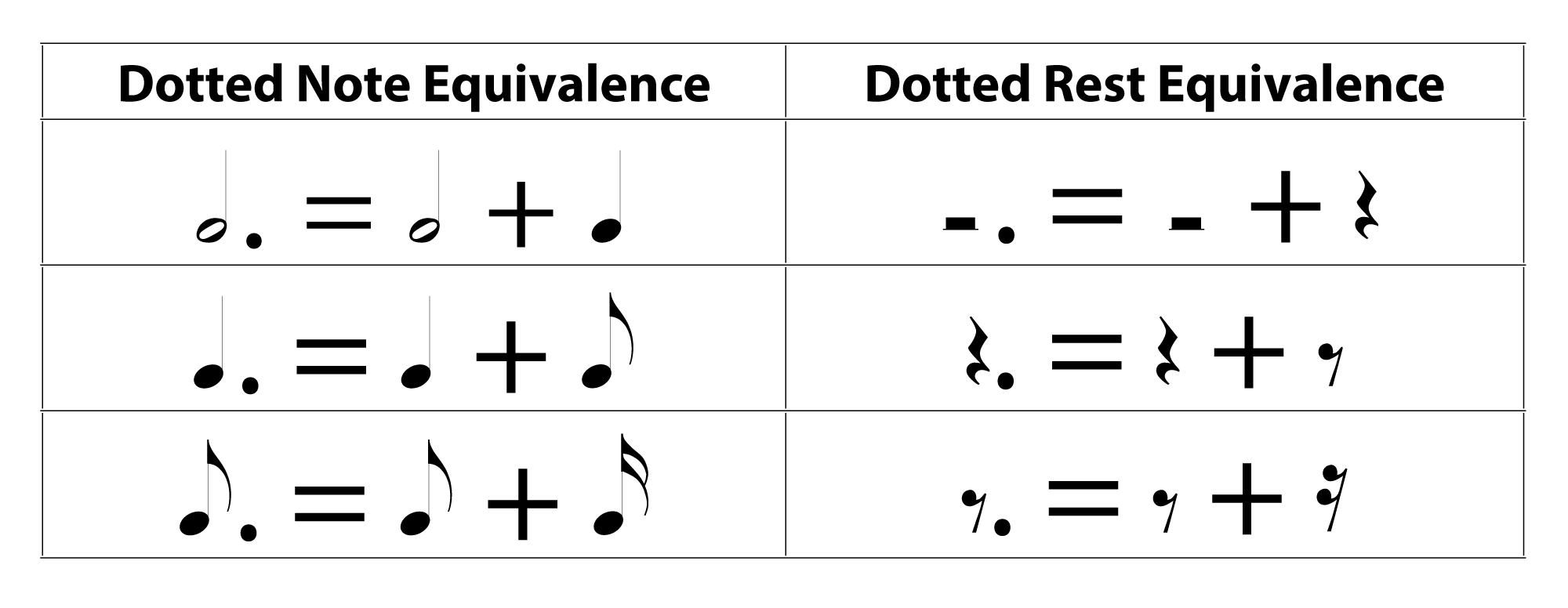
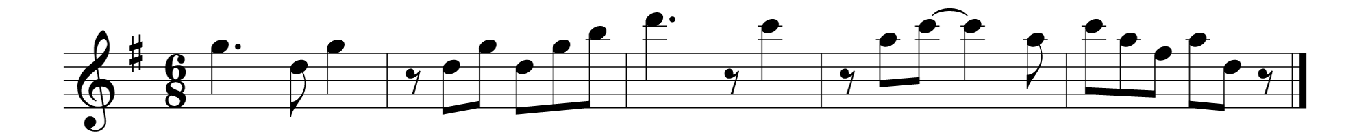
A dot placed after a note or rest increases its duration by one-half of its original value. This is shown in Table 3.6. Figure 3.18 shows a fragment of Mozart’s “A Little Night Music,” which contains eighth rests in the second, third, and fourth measures. Since this piece is in $$\frac{6}{8}$$ time, the eighth rest gets one beat.

3.1.5.5 Key Signature

Many words in the field of music and sound are overloaded – that is, they have different meanings in different contexts. The word “key” is one of these overloaded terms. Thus far, we have been using the word “key” to denote a physical key on the piano keyboard. (For the discussion that follows, we’ll call this kind of key a “piano key.”) There’s another denotation for key that relates to diatonic scales, both major and minor. In this usage of the word, a key is a group of notes that constitute a diatonic scale, whether major or minor.

Each key is named by the note on which it begins. The beginning note is called the key note or tonic ( tonal center) note. If we start a major diatonic scale on the piano key of C, then following the pattern 2 2 1 2 2 2 1, only white keys are played. This group of notes defines the key of C major. Now consider what happens if we start on the note D. If you look at the keyboard and consider playing only white keys starting with D, you can see that the pattern would be 2 1 2 2 2 1 2, not the 2 2 1 2 2 2 1 pattern we want for a major scale. Raising F and C each by a semitone – that is, making them F# and C# – changes the pattern to 2 2 1 2 2 2 1. Thus the notes D, E, F#, G, A, B, C# and D define the key of D. By this analysis, we see that the key of D requires two sharps – F and C. Similarly, if we start on D and follow the pattern for a minor diatonic scale – 2 1 2 2 1 2 2 – we play the notes D, E, F, G, A, B♭, and D. This is the key of D minor.

Each beginning note (tonic note) determines the number of sharps or flats that are played in the 2 2 1 2 2 2 1 scale for a major key or in the 2 1 2 2 1 2 2 sequence for a minor key. Beginning an octave on the piano key C implies you’re playing in the key of C and play no sharps or flats for C major. Beginning a scale on the piano key D implies that you’re playing in the key of D and play two sharps for D major.

Let’s try a similar analysis on the key of F. If you play a major scale starting on F using all white keys, you don’t get the pattern 2 2 1 2 2 2 1. The only way to get that pattern is to lower the fourth note, B, to B♭. Thus, the key of F major has one flat. The key of F minor has four flats – A♭, B♭, D♭, and E♭, as you can verify by following the sequence 2 1 2 2 1 2 2 starting on F.

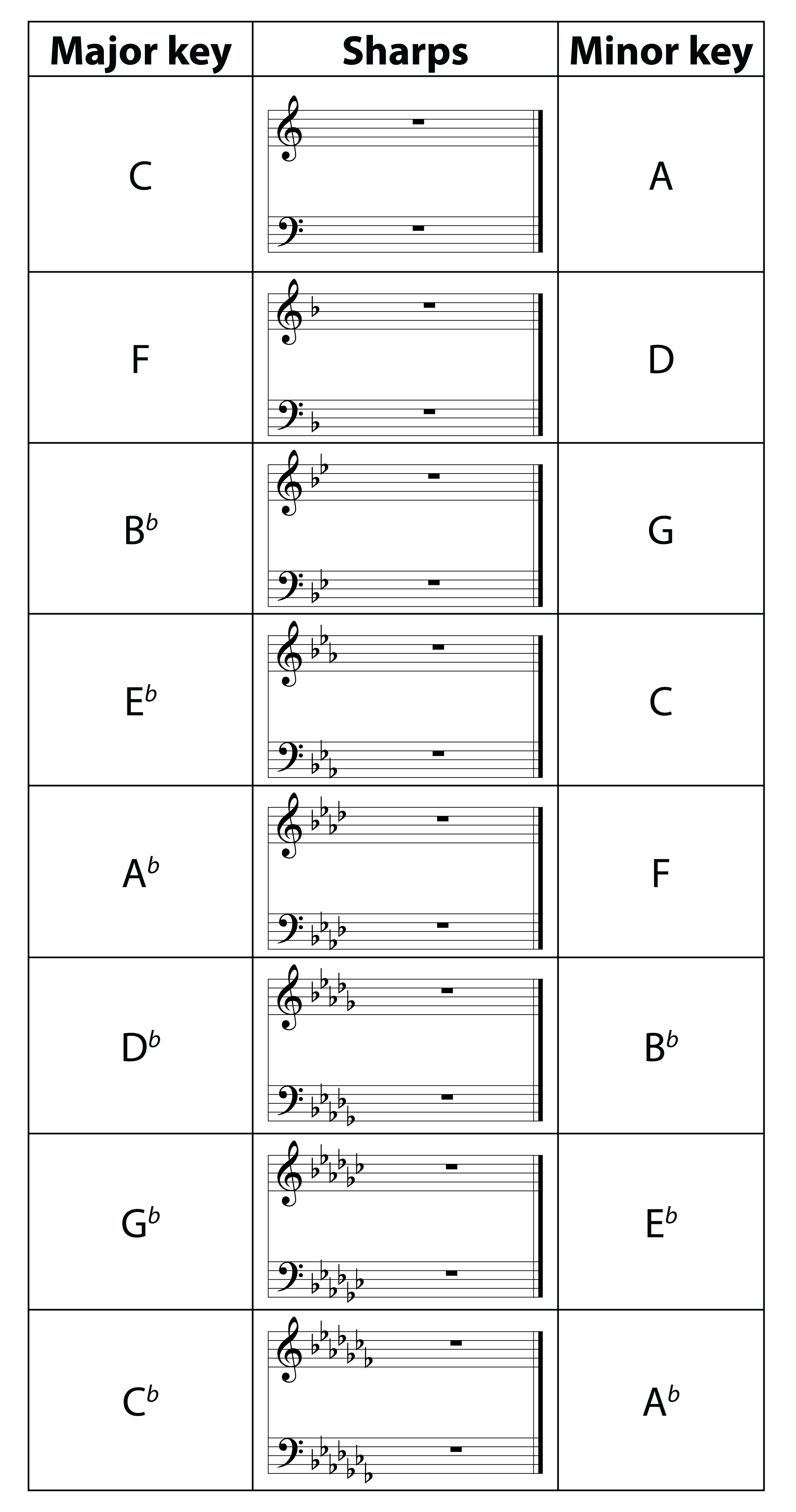
Like meter, the key of a musical composition is indicated at the beginning of each staff, in the key signature. The key signature indicates which notes are to be played as sharps or flats. The key signatures for all the major keys with sharps are given in Table 3.7. The key signatures for all the major keys with flats are given in Table 3.8.

You may have noticed that the keys of F major and D minor have the same key signature, each having one flat, B♭. So when you see the key signature for a musical composition and it has one flat in it, how do you know if the composition is written in F major or D minor, and what difference does it make? One difference lies in which note feels like the “home” note, the note to which the music wants to return to be at rest. A composition in the key of F major tends to begin and end in F. The use of specific chords reinforces the key, also. A second difference is a subjective response to major and minor keys. Minor keys generally sound more somber, sad, or serious while major keys are bright and happy to most listeners.

You can see in the tables below that each major key has a relative minor key, as indicated by the keys being in the same row in the table and sharing a key signature. Given a major key k, the relative minor is named by the note that is three semitones below k. For example, A is three semitones below C, and thus A is the relative minor key with respect to C major. When keys are described, if the words “major” and “minor” are not given, then the key is assumed to be a major key.

You’ve seen how, given the key note, you can determine the key signature for both major and minor keys. So how do you work in reverse? If you see the key signature, how can you tell what key this represents? A trick for major keys is to name the note that is one semitone above the last sharp in the key signature. For example, the last sharp in the second key signature in Table 3.7 is F#. One semitone above F# is G, and thus this is the key of G major. For minor keys, you name the note that is two semitones below the last sharp in the key signature. For the first key signature in Table 3.7, the last sharp is F#. Two semitones below this is the note E. Thus, this is also the key signature for E minor.

To determine a major key based on a key signature with flats, you name the note that is five semitones below the last flat. In the key that has three flats, the last flat is A♭. Five semitones below that is E♭, so this is the key of E♭major. (This turns out to be the next to last flat in each key with at least two flats.) To determine a minor key based on a key signature with flats, you name the note that is four semitones above the last flat. Thus, the key with three flats is the key of C minor. (You could also have gotten this by going three semitones down from the relative major key.)

The key signature for a harmonic minor key is the same as the natural minor. To create the pattern [2 1 2 2 1 3 1] (harmonic minor) from [2 1 2 2 1 2 2] (natural minor), the seventh scale degree is raised by a semitone. Since the natural minor’s key signature is being used, sharps or naturals are needed on individual notes to create the desired pattern of whole tones and semitones for the harmonic minor. The scale for a example harmonic minor is notated as shown in Figure 3.19. (In this section and following ones, we won’t include measures and time signatures when they are not important to the point being explained.)

Similarly, the melodic minor uses the key signature of the natural minor. Then adjustments have to be made in both the ascending and descending scales to create the melodic minor. To create the ascending pattern [2 1 2 2 2 2 1] (melodic minor) from [2 1 2 2 1 2 2] (natural minor), it suffices to raise both the sixth and seventh note by a semitone. This is done by adding sharps or naturals as necessary, depending on the key signature. The descending pattern for a melodic minor is the same as for the natural minor – [2 2 1 2 2 1 2]. Thus, the notes that are raised in the ascending scale have to be returned to their natural minor position for the key by adding flats, or naturals, as necessary. This is because once an accidental is added in a measure, it applies to the note to which it was added for the remainder of the measure.

F minor melodic is notated as shown in Figure 3.20. In F minor melodic, since D and E are normally flat for that key, a natural is added to each to remove the flat and thus move them up one semitone. Then in the descending scale, the D and E must explicitly be made flat again with the flat sign.

In E minor melodic, a sharp is added to the sixth and seventh notes – C and D – to raise them each as semitone. Then in the descending scale, the D and E must explicitly be made natural again with the sign, as shown in Figure 3.21.

3.1.5.6 The Circle of Fifths

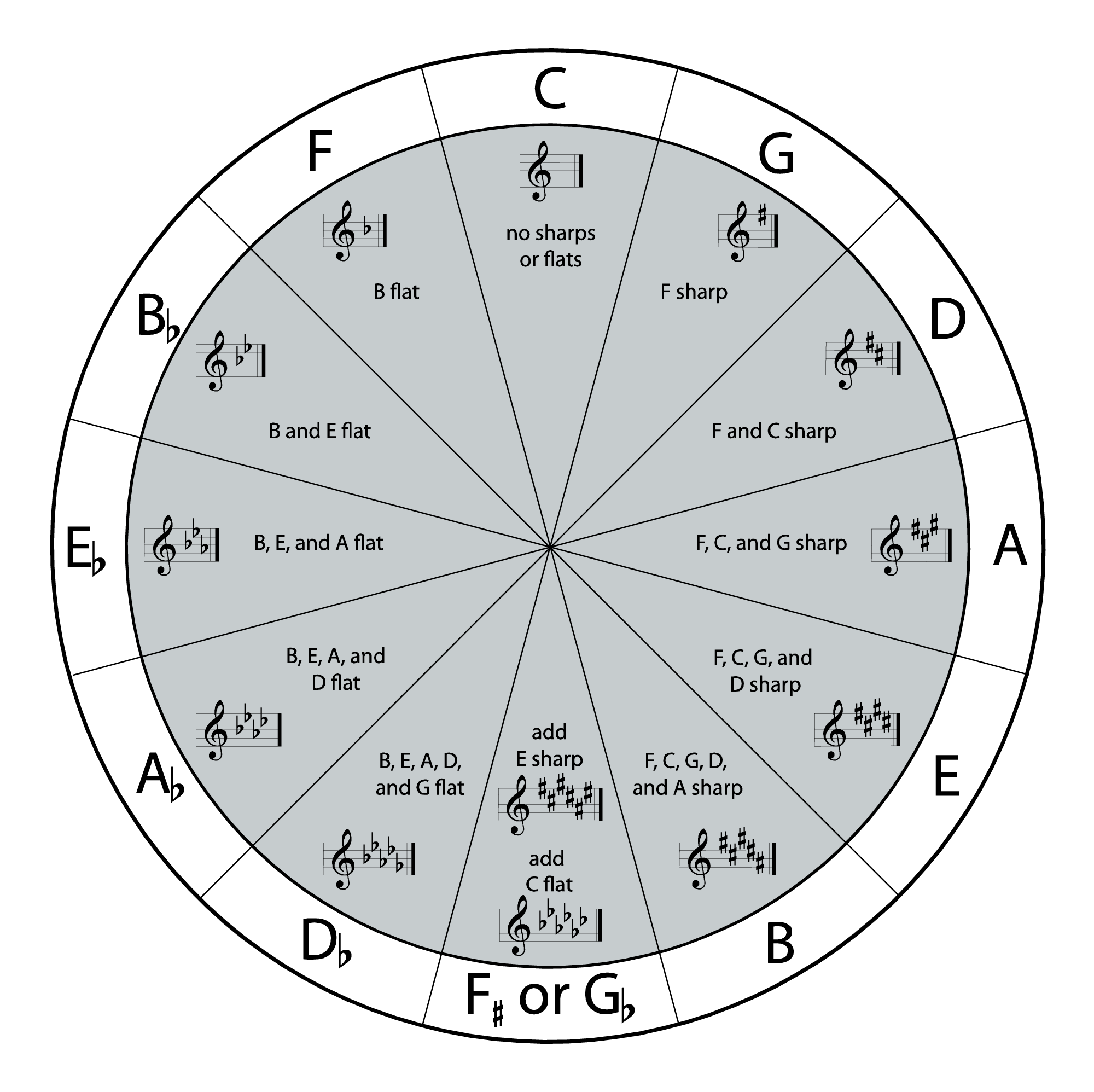
In Section 3.1.5, we showed how keys are distinguished by the sharps and flats they contain. One way to remember the keys is by means of the circle of fifths, a visual representation of the relationship among keys. The circle is shown in Figure 3.22. The outside of the circle indicates a certain key. The inner circle tells you how many sharps or flats are in the key.

[wpfilebase tag=file id=110 tpl=supplement /]

A fifth is a type of interval. We’ll discuss intervals in more detail in Section 3.1.6.2, but for now all you need to know that a fifth is a span of notes that includes five lettered notes. For example, the notes A, B, C, D, and E comprise a fifth, as do C, D, E, F, and G.

If you start with the key of C and move clockwise by intervals of fifths (which we call “counting up”), you reach successive keys each of which has one more sharp than the previous one – the keys of G, D, A, and so forth. For example, starting on C and count up a fifth, you move through C, D, E, F, and G, five lettered notes comprising a fifth. Counting up a fifth consists of moving up seven semitones – C to C#, C# to D, D to D#, D# to E, E to F, F to F#, and F# to G. Notice that on the circle, moving clockwise, you’re shown G as the next key up from the key of C. The key of G has one sharp. The next key up, moving by fifths, is the key of D, which has two sharps. You can continue counting up through the circle in this manner to find successive keys, each of which has one more sharp than the previous one.

Starting with the key of C and moving counterclockwise by intervals of fifths (“counting down”), you reach successive keys each of which has one more flat than the previous one – the keys of F, B♭, E♭, and so forth. Counting down a fifth from C takes you through C, B, A, G, and F – five lettered notes taking you through seven semitones, Counting down a fifth from F takes you through F, E, D, C, and B. However, since we again want to move seven semitones, the B is actually B♭.   The seven semitones are F to E, E to E♭, E♭ to D, D to D♭, D♭ to C, C to B, and B to B♭. Thus, the key with two flats is the key of B♭.

[wpfilebase tag=file id=111 tpl=supplement /]

The keys shown in the circle of fifths are the same keys shown in Table 3.7 and Table 3.8. Theoretically, Table 3.7 could continue with keys that have seven sharps, eight sharps, and on infinitely. Moving the other direction, you could have keys with seven flats, eight flats, and on infinitely. These keys with an increasing number of sharps would continue to have equivalent keys with flats. We’ve shown in Figure 3.22 that the key of F#, with six sharps, is equivalent to the key of G♭, with six flats. We could have continued in this manner, showing that the key of C#, with seven sharps, is equivalent to the key of D♭, with five flats. Because the equivalent keys go on infinitely, the circle of fifths is sometimes represented as a spiral. Practically speaking, however, there’s little point in going beyond a key with six sharps or flats because such keys are harmonically the same as keys that could be represented with fewer accidentals. We leave it as an exercise for you to demonstrate to yourself the continued key equivalences.

3.1.5.7 Key Transposition

[wpfilebase tag=file id=112 tpl=supplement /]

All major keys have a similar sound in that the distance between neighboring notes on the scale follows the same pattern. One key is simply higher or lower than another. The same can be said for the similarity of minor keys. Thus, a musical piece can be transposed from one major (or minor) key to another without changing its composition. A singer might prefer one key over another because it is in the range of his or her voice.

Figure 3.23 shows the first seven notes of “Twinkle, Twinkle Little Star,” right-hand part only, transposed from the key of C major to the key of E major. If you play these on a keyboard, you’ll hear that C major and E major sound the same, except that the second is higher than the first.

3.1.6.1 Historical Context

For as far back in history as we can see, we find evidence that human beings have made music. We know this from ancient drawings of lutes and harps, Biblical references to David playing the lyre for King Saul, and the Greek philosopher Pythagoras’s calculation of harmonic intervals. The history of music and musical styles is a fascinating evolution of classical forms, prescriptive styles, breaks from tradition, and individual creativity. An important thread woven through this evolution is the mathematical basis of music and its relationship with beauty.

In the 6^th century BC, the Greek philosopher Pythagoras recognized the mathematical basis of harmony, noting how the sound of a plucked string changes in proportion to the length of the string. However, harmony was not the most important element of music composition as it developed through the Middle Ages. The chanting of medieval monks evolved in a variety of styles and modalities. The early chants, called plainchant, were essentially syllabically-accented speech. Later styles involved two to eight monks chanting multiple melodic lines, traditionally with no instrumental accompaniment and in different musical modes. Madrigals of the Middle Ages were composed of single solo lines with simple instrumental accompaniment. In the Baroque period, multiple independent strands became interwoven in a style called polyphony, which reached its zenith in the fugues, canons, and contrapuntal compositions of Johann Sebastian Bach. Although we have come to think of harmony as an essential element of music, its music-theoretic development and its central position in music composition didn’t begin in earnest until the 18^th century, spurred by Jean-Philippe Rameau’s Treatise on Harmony.

In this chapter, we emphasize the importance of harmony in musical composition because it is an essential feature of modern Western music. However, we acknowledge that perceptions of what is musical vary from era to era and culture to culture, and we can give only a small part of the picture here. We encourage the reader to explore other references on the subject of music history and theory for a more complete picture.

3.1.6.2 Intervals

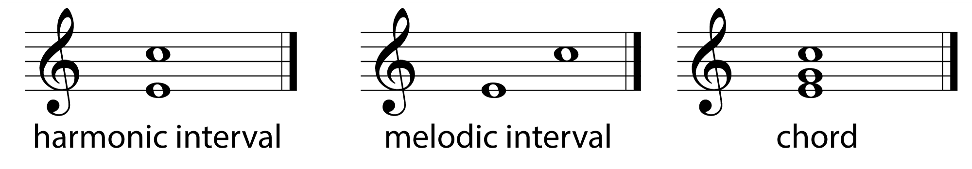
An understanding of melody and harmony in Western music composition begins with intervals. An interval is the distance between two notes, measured by the number of lettered notes it contains counting both the starting and ending notes. If the notes are played at the same time, the interval is a harmonic interval. If the notes are played one after the other, it is a melodic interval. If there are at least three notes played simultaneously, they constitute a chord. When notes are played at the same time, they are stacked up vertically on the staff. Figure 3.24 shows a harmonic interval, melodic interval, and chord.

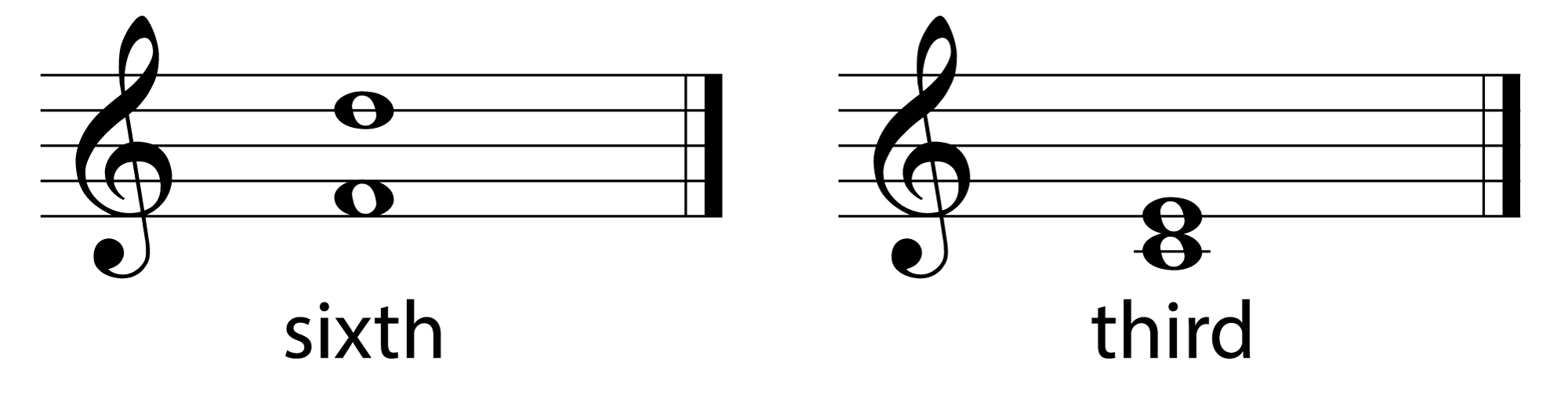
Intervals are named by the number of lettered notes from the lowest to highest, inclusive. The name of the interval can be expressed as an ordinal number. For example, if the interval begins at F and ends in D, there are six lettered notes in the interval, F, G, A, B, C, and D. Thus, this interval is called a sixth. If the interval begins with C and ends in E, it is called a third, as shown in Figure 3.25 Note that in this regard the presences of sharps or flats isn’t significant. The interval between F and D is a sixth, as is the interval between F and D#.

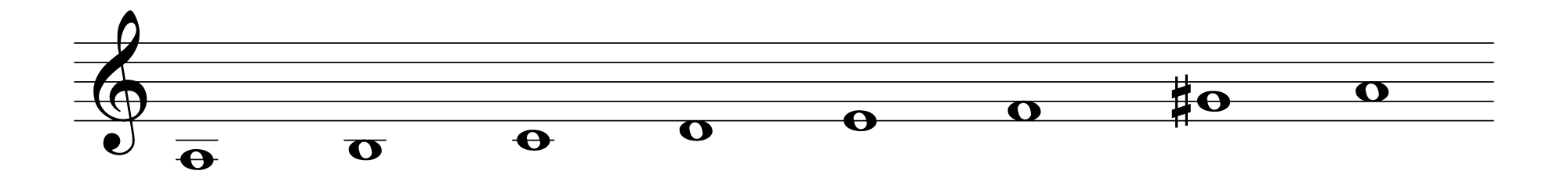
Because there are eight notes in an octave, with the last letter repeated, there are eight intervals in an octave. These are shown in Figure 3.26, in the key of C. Each interval is constructed in turn by starting on the key note and moving up by zero lettered notes, one lettered note, two lettered notes, and on up to eight lettered notes. Moving up one lettered note means moving up to the next line or space on the staff.

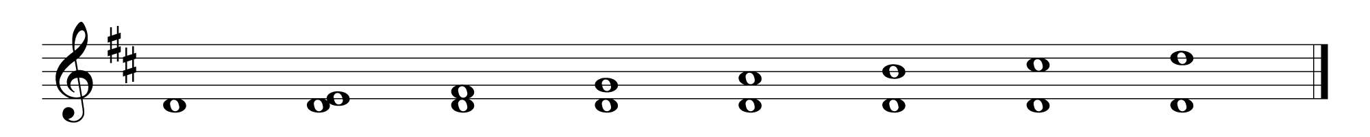
The same intervals can be created in any key. Consider the key of D. Unison is simply one note. A second is D an E. A third is D and F#. A fourth is D and G. A fifth is D and A. A sixth is D and B. A seventh is D and C#. These intervals are shown in Figure 3.27. Note that F and C are implicitly sharp in this key.

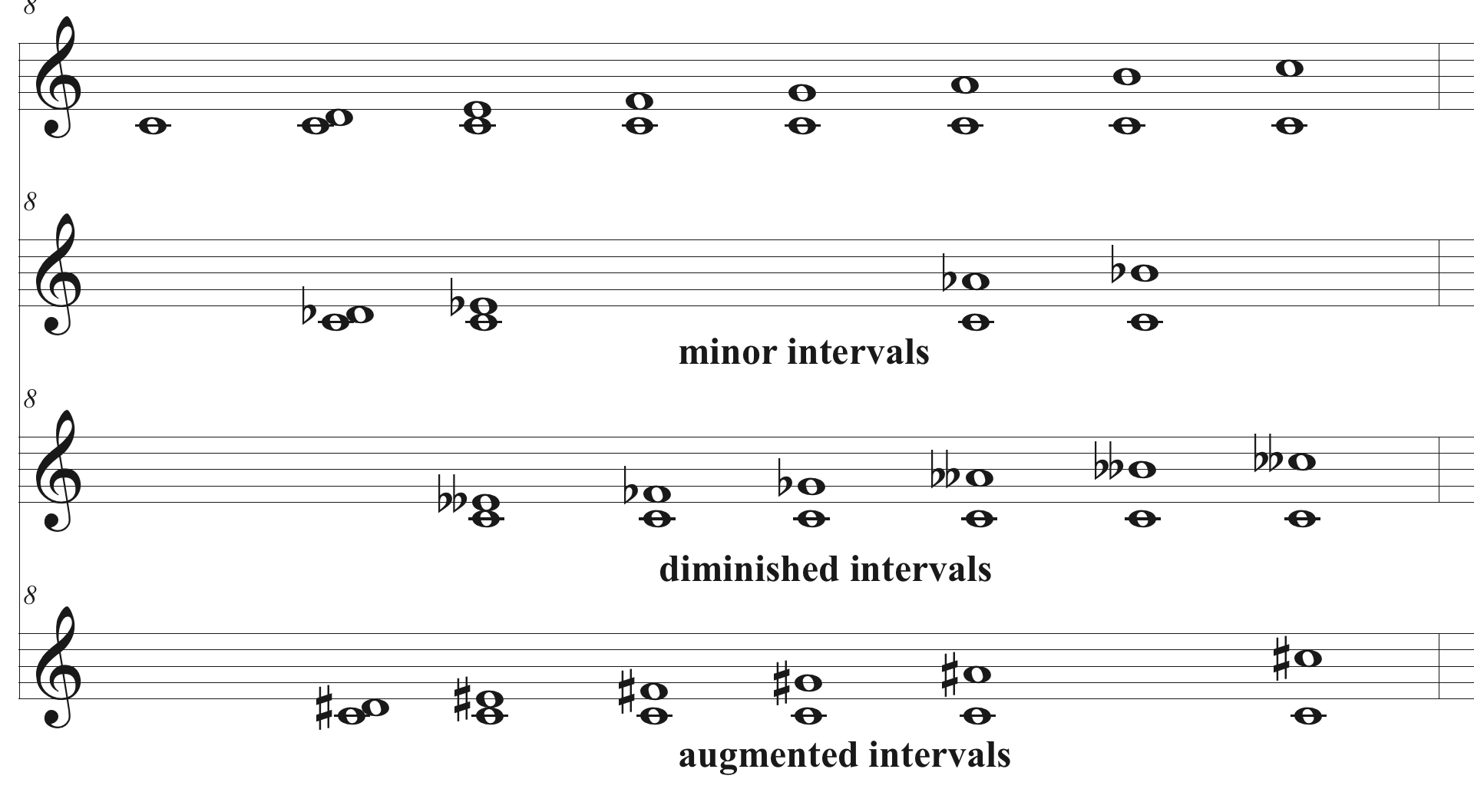
Intervals are named not only by their size but also by quality — major, perfect, minor, augmented, and diminished. A full discussion of the intervals qualities is beyond the scope of this book. We’ll introduce you to them by showing examples and explaining a little about how they relate to each other. (See Figure 3.28.)

A major interval is considered major if the second note of the interval is in the diatonic scale of a major scale beginning at the first note of the interval. For example,  C and G constitute a major interval because G is a note in the key of C.

A major interval can be converted to a minor interval by lowering the higher note one semitone.

The intervals that cannot be made minor are called perfect. (They cannot be made minor because lowering the top note by a semitone creates a different interval. (For example, consider lowering the G in the C-G fifth by a semitone. Then the top note is an F, the interval becomes a fourth instead of a fifth.) The perfect intervals are perfect unison, the fourth, the fifth, and the octave.

Two other types of intervals exist: diminished and augmented. A diminished interval is one semitone smaller than a perfect interval or two semitones smaller than a major interval. An augmented interval is one semitone larger than a perfect or major interval.   All the intervals for the key of C are shown in Figure 3.28. The intervals for other keys could be illustrated similarly.

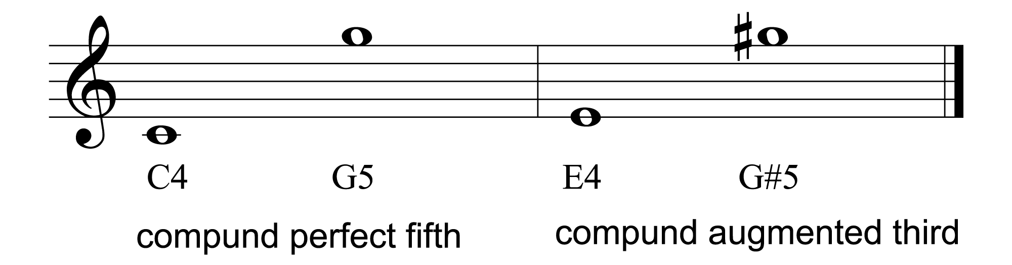
You can create a compound interval by taking any of the interval types defined above and moving the upper note up by one or more octaves. If you’re trying to identify intervals in a score, you can count the number of lettered notes from the beginning to the end of the interval and “mod” that number by 7. The result gives you the type of interval. For example, if the remainder is 3, then the interval is a third. The mod operation divides by an integer and gives the remainder. This is the same as repeatedly subtracting 7 (the number of notes in an octave, not counting the repeat of the first note an octave higher) until you reach a number that is less than 7. Figure 3.29 shows examples of two compound intervals. The first goes from C4 to G5, a span of 12 notes. 12 mod 7 = 5, so this is a compound perfect fifth.   The second interval goes from E4 to G5#, a span of 10 notes. 10 mod 7 = 3, so this is a compound third. However, because the G is raised to G#, this is, more precisely, a compound augmented third.

Intervals can be characterized as either consonant or dissonant. Giving an oversimplified definition, we can say that sounds that are pleasing to the ear are called consonant, and those that are not are called dissonant. Of course, these qualities are subjective. Throughout the history of music, the terms consonant and dissonant have undergone much discussion. Some music theorists would define consonance as a state when things are in accord with each other, and dissonance as a state of instability or tension that calls for resolution. In Section 3.3.2, we’ll look more closely at a physical and mathematical explanation for the subjective perception of consonance as it relates to harmony.

[wpfilebase tag=file id=34 tpl=supplement /]

Intervals help us to characterize the patterns of notes in a musical composition. The musical conventions from different cultures vary not only in their basic scales but also in the intervals that are agreed upon as pleasing to the ear. In Western music of our times, the perfect intervals, major and minor thirds, and major and minor sixths are generally considered consonant, while the seconds, sevenths, augmented, and diminished intervals are considered dissonant. The consonant intervals come to be used frequently in musical compositions of a culture, and the listener’s enjoyment is enhanced by a sense of recognition. This is not to say that dissonant intervals are simply ugly and never used. It is the combination of intervals that makes a composition. The combination of consonant and dissonant intervals gives the listener an alternating sense of tension and resolution, expectation and completion in a musical composition.

3.1.6.3 Chords

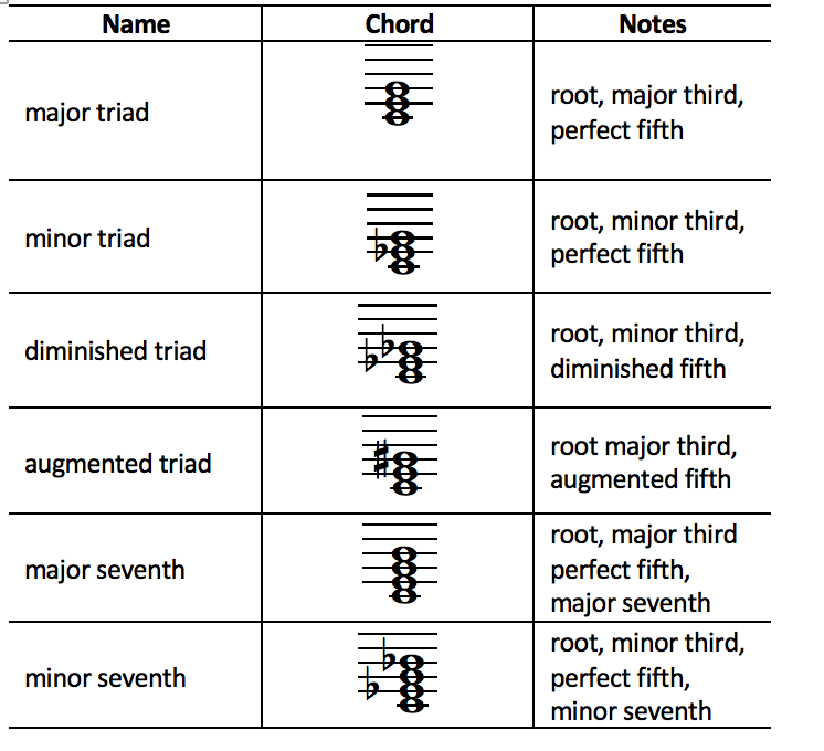
A chord is three or more notes played at the same time. We will look at the most basic chords here – triads, which consist of three notes stacked vertically in thirds, creating tertian harmony .

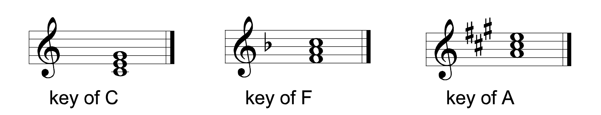
Triads can be major, minor, diminished, or augmented. The lowest note of a triad is its root. In a major triad, the second note is a major third above the root, and the third note is a perfect fifth above the root. In the root position of a triad in a given key, the tonic note of the key is the root of the triad. (Refer to Table 3.2 for the names of the notes in a diatonic scale.) The major triads for the keys of C, F, and A are shown in root position in Figure 3.30.

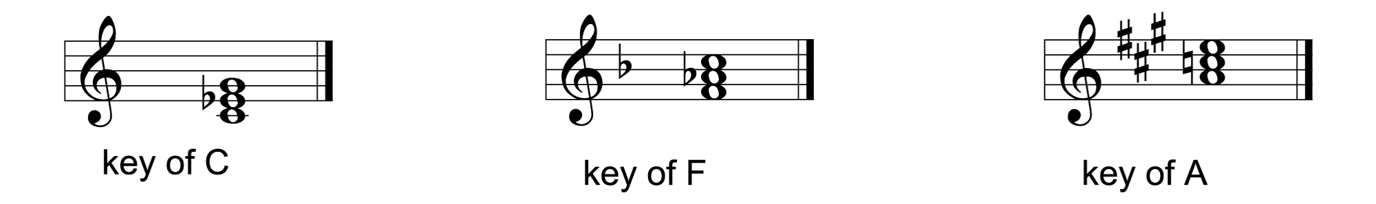
In a minor triad, the second note is a diatonic minor third above the root, and the third note is a diatonic perfect fifth above the root. The minor triads for the keys of C, F, and A are shown in root position in Figure 3.31.

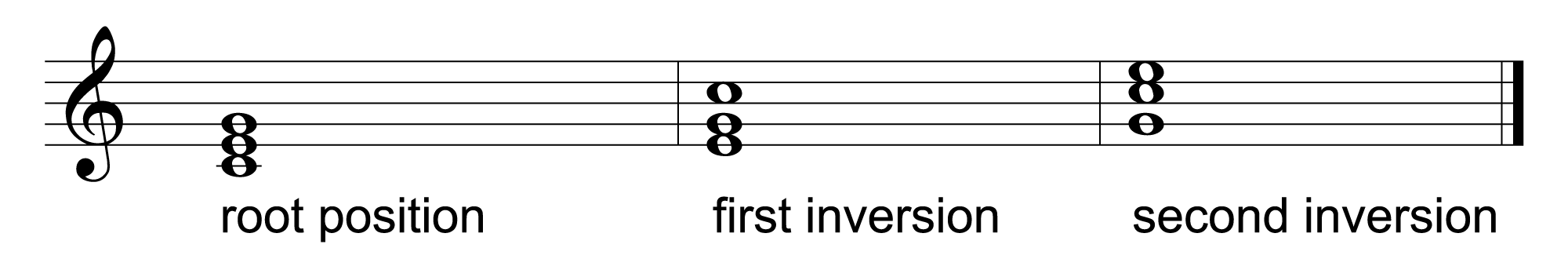
Chords can be inverted by rotating the notes up or down – in other words, making the 3^rd or the 5^th the bottom or lowest note. In the first inversion, the lowest note is the 3^rd, and in the second inversion, the lowest note is the 5^th. In the second inversion, the mediant of the key becomes the root and the tonic is moved up an octave. In the third inversion, the dominant of the key becomes the root, and both the mediant and tonic are moved up an octave. The first and inversions are shown in Figure 3.32.

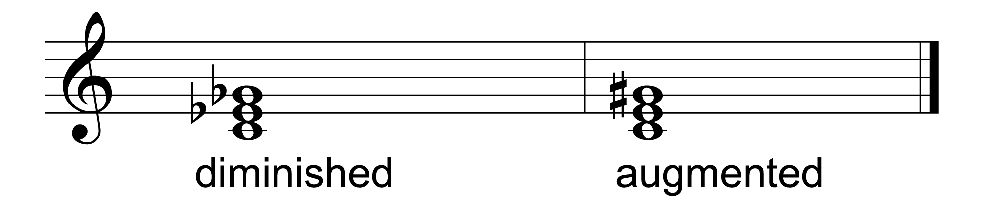
A diminished triad has a root note followed by a minor third and a diminished fifth. An augmented triad has a root note followed by a major third and an augmented fifth. The diminished and augmented triads for the key of C are shown in Figure 3.33.

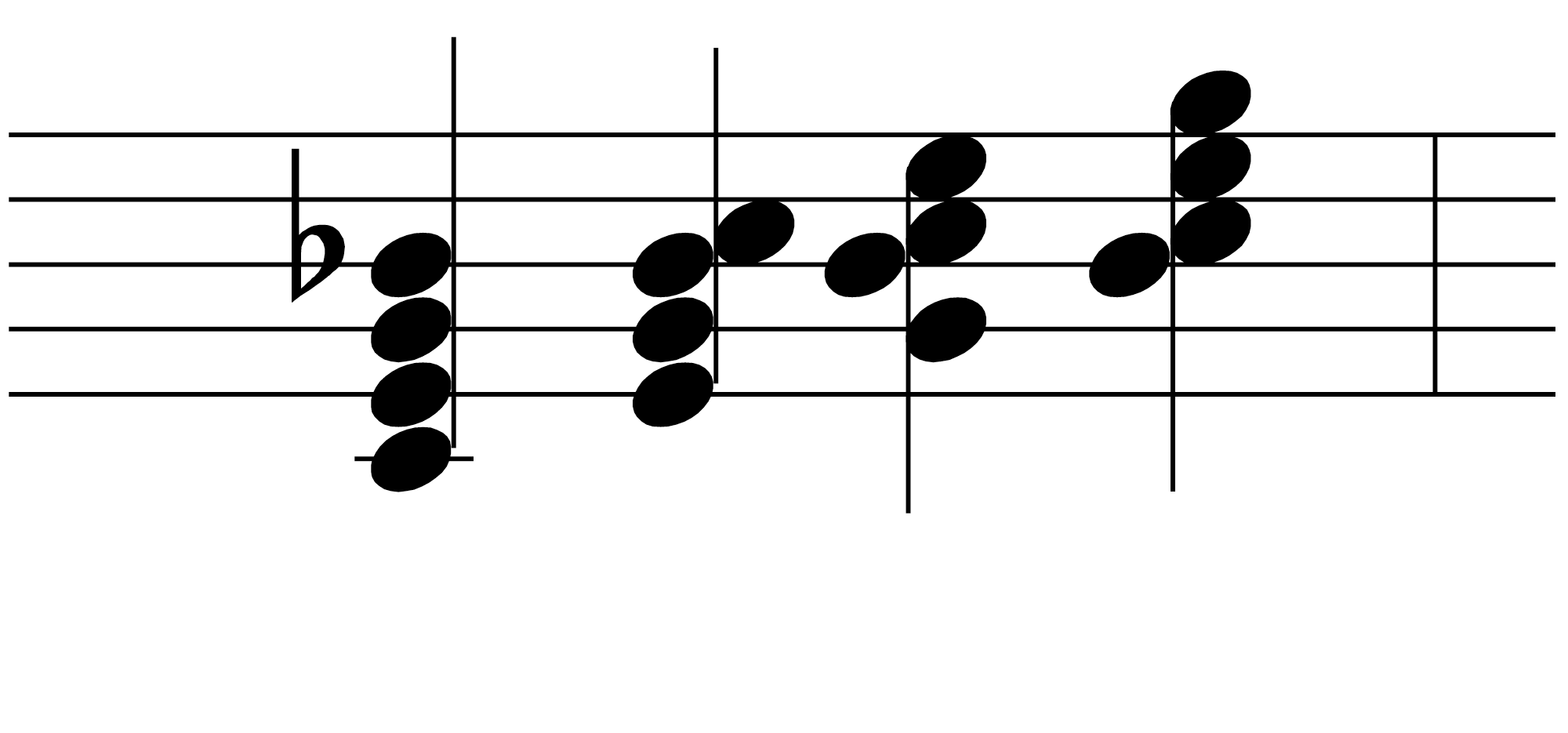
We’ve looked at only triads so far. However, chords with four notes are also used, including the major, minor, and dominant sevenths. The major seventh chord consists of the root, major third, perfect fifth, and major seventh. The minor seventh consists of the root, minor third, perfect fifth, and minor seventh. The dominant seventh consists of the root, major third, perfect fifth, and minor seventh.   Dominant chords have three inversions. The dominant seventh for the key of C is shown with its inversions in Figure 3.34. (Note that B is flat in all the inversions.)

Thus we have seven basic chords that are used in musical compositions. These are summarized in Table 3.9.

[wpfilebase tag=file id=113 tpl=supplement /]

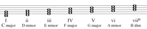
All major keys give rise to a sequence of triads following the same pattern. To see this, consider the sequence you get in the key of C major by playing a triad starting on each of the piano keys in the scale. These triads are shown in Figure 3.35. Each is named with the name of its root note. (Note that we use the convention where upper case Roman numerals are used for major chords and lower case are used to minor chords. =)

[wpfilebase tag=file id=114 tpl=supplement /]

Each of the chords in this sequence can be characterized based on its root note. Triad I is easy to see. The first note is C and it’s a major triad, so it’s C major. Triad ii starts on D, so consider what kind of triad this would be in the key of D. It has the notes D, F, and A. However, in the key of D, F should be sharp. D is not sharp in the triad ii shown, so this is a minor triad from the key of D. Triad iii has the notes E, G, and B. In the key of E, G is sharp, but in the triad iii shown, it is not. Thus, the third triad in the key of C is E minor. Let’s skip to vii°, which has the notes B, D, and F. In the key of B, the notes D and F are sharp, but they’re not in triad vii. This makes vii° a B diminished. By this analysis, we can determine that the sequence of chords in C major is C major, D minor, E minor, F major, G major, A minor, and B diminished.

All major keys have this same sequence of chord types – major, minor, minor, major, major, minor, and diminished.  For example, the key of D has the chords D major, E minor, F# minor, G major, A major, B minor and C# diminished. We refer you to a music theory textbook for a similar analysis of chords in a minor key.

[table caption=”Table 3.10 Types of triad chords in major and minor keys” width=”80%” colalign=”center|center|center”]

Chord~~number in~~major key,Chord~~type in major key, Chord number in~~minor key,Chord type~~inminor key

I,major,i,minor

ii,minor,ii°,diminished

iii,minor,III,major

IV,major,vi,minor

V,major,V,major

vi,minor,VI,major

vii°,diminished,vii°,diminished

[/table]

3.1.6.4 Chord Progressions

So what is the point of identifying and giving names to intervals and chords? The point is that this gives us a way to analyze music, communicate about it, and compose it in a way that yields a logical order and an aesthetically pleasing form within a style. When chords follow one another in certain progressions, they provoke feelings of tension and release, expectation and satisfaction, conflict and resolution. This emotional rhythm is basic to music composition.

Let’s look again at the chords playable in the key of C, as shown in Figure 3.35. Chord progressions can be represented by a sequence of Roman numerals that correspond to the scale degree (1 to 7) for the root note of the chord. For example, the right-hand part of “Twinkle, Twinkle Little Star” in the key of C major, shown in Figure 3.23, could be accompanied by the chords I   I   IV   I   IV   I   V   I in the left hand, as shown in Figure 3.36. This chord progression is in fact a very common pattern.

You can play this yourself with reference to the triads from the key of C major, shown in Figure 3.35. However, to make the chords sound more interesting, you can invert them so that the lowest note leads more smoothly to the next chord’s lowest note (bass note). A beginning piano student may invert chords to make them easier to play. For example, chord I can be played as C, E, G; chord IV as C, F, A (2^nd inversion); and chord V as B, D, G (1^st inversion), as shown in Figure 3.37.

A simple way of looking at chord progressions is based on tonality – a system for defining the relationships of chords based on the tonic note for a given key. Recall that the tonic note is the note that begins the scale for a key. In fact, the key’s name is derived from the tonic note. In the key of C, the tonic note is C. Triad I is the tonic triad because it begins on the tonic note. You can think of this as the home chord, the chord where a song begins and to which it wants to return. Triad V is called the dominant chord. It has this name because chord progressions in a sense pull toward the dominant chord, but then tend to return to the home chord, chord I. Returning to chord I gives a sense of completion in a chord progression, called a cadence. The progression from I to V and back to I again is called an authentic cadence because it is the clearest example of tension and release in a chord progression. It is the most commonly used chord progression in modern popular music, and probably in Western music as a whole.

Another frequently used progression moves from I to IV and back to I. IV is the subdominant chord, named because it serves as a counterbalance to the dominant. The I IV I progression is called the plagal cadence. Churchgoers may recognize it as the sound of the closing “amen” to a hymn. Together, the tonic, subdominant, and dominant chords and their cadences serve as foundational chord progressions. You can see this in “Twinkle, Twinkle Little Star,” a tune for which Wolfgang Amadeus Mozart wrote twelve variations.

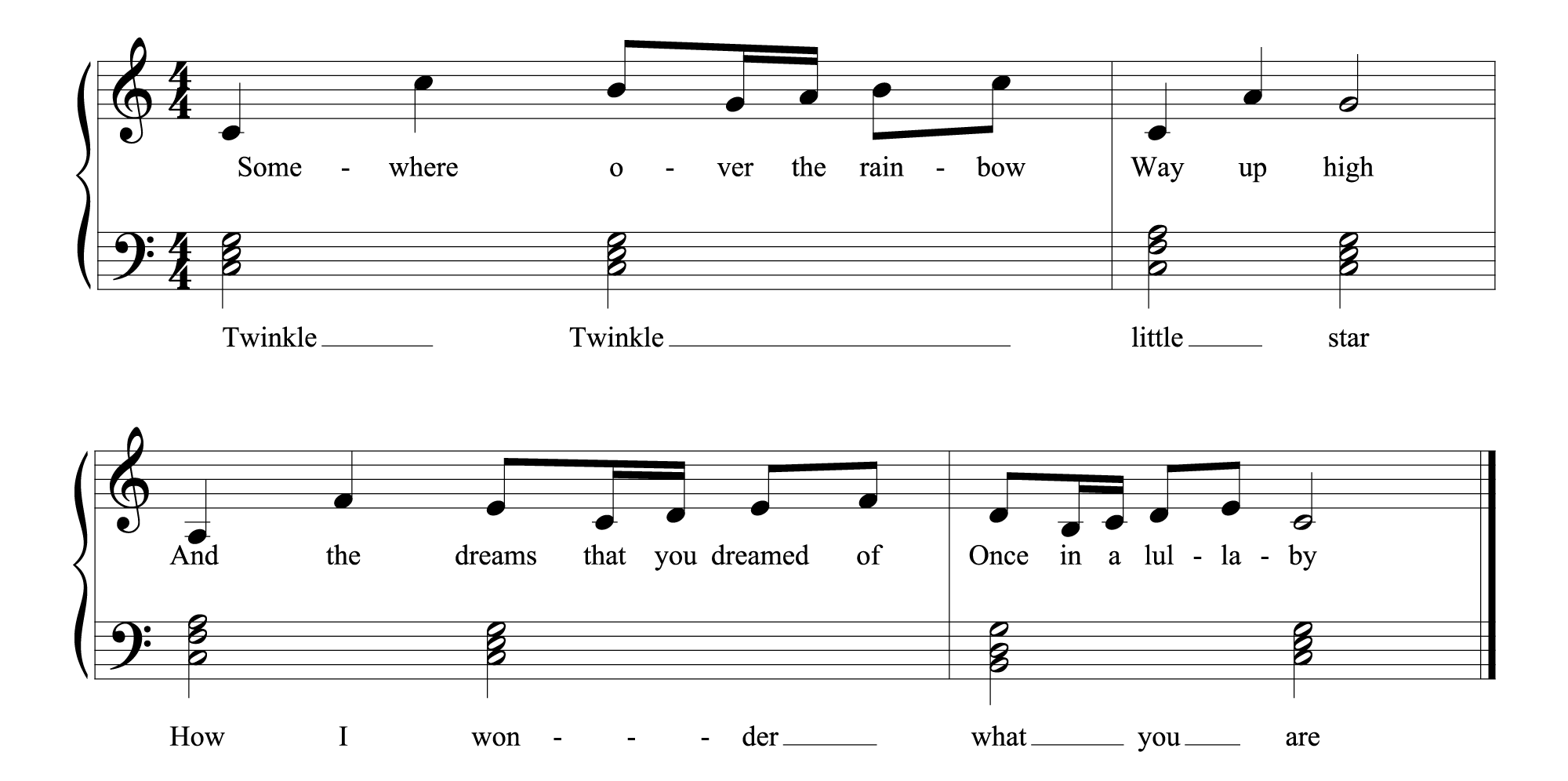
The perfect and plagal cadences are commonly used chord progressions, but they’re only the tip of the iceberg of possibilities. “Over the Rainbow” from The Wizard of Oz, with music written by Harold Arlen, is an example of how a small variation from the chord progression of “Twinkle, Twinkle Little Star” can yield beautiful results. If you speed up the tempo of “Over the Rainbow”, you can play it with the same chords as are used for “Twinkle, Twinkle Little Star,” as shown in Figure 3.38. The only one that sounds a bit “off” is the first IV.

[wpfilebase tag=file id=139 tpl=supplement /]

[wpfilebase tag=file id=140 tpl=supplement /]

Learning to read music on a staff is important for anyone working with music. However, for non-musicians working on computer-based music, there are other, perhaps more intuitive ways to picture musical notes — e.g., by means of MIDI.

MIDI (Musical Instrument Digital Interface) is a protocol designed for encoding and exchange of musical information. (MIDI is introduced in Chapter 1, and we’ll talk more about MIDI in Chapters 5 and 6, but what follows will give you a preview of graphical user interfaces between MIDI and the user.) MIDI uses computer-based synthesizers and samplers to turn the encoding into digital audio that can be played through the computer’s sound card. A MIDI sequencer is the software interface between the user and the MIDI samplers and synthesizers. MIDI sequencers enable the computer to receive, store, modify, and play MIDI data. Sequencers provide two views of music that you may find helpful if you can’t read music on a musical staff – the piano roll view and the event list view.

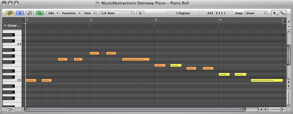
A piano roll view is essentially a graph with the vertical axis representing the notes on a piano and the horizontal axis showing time. In Figure 3.41 you can see a graphical representation of a piano keyboard flipped vertically and placed on the left side of the window. On the horizontal row at the top of the window you can see a number representing each new measure. This graph forms a grid where notes can be placed at the intersection of the note and beat where the note should occur. Notes can also be adjusted to any duration. In this case, you can see each note starting on a quarter beat. Some notes are longer than others. The quarter notes are shown using bars that start on a quarter beat but don’t extend beyond the neighboring quarter beat. The half notes start on a quarter beat and extend beyond the neighboring quarter beat. In most cases you can grab note events using your mouse pointer and move them to different notes on the vertical scale as well as move them to a different beat on the grid. You can even extend or shorten the notes after they’ve been entered. You can also usually draw new notes directly into the piano roll.

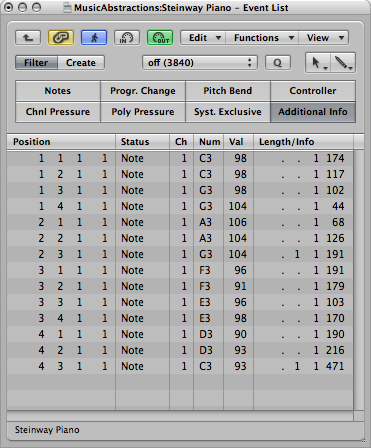
Another way you might see the musical data is in an event list view, as shown in Figure 3.42. This is a list showing information about every musical event that occurs for a given song. Each event usually includes the position in time that the event occurs, the type of event, and any pertinent details about the event such as note number, duration, etc. The event position value is divided into four columns. These are Bars:Beats:Divisions:Ticks. You should already be familiar with bars and beats. Divisions are some division of a beat. This is usually an eighth or asixteenth and can be user-defined. Ticks are a miniscule value. You can think of these like frames or milliseconds. The manual for your specific software will give you its specific for time value of ticks.

You can edit events in an event list by changing the properties, and you can add and delete events in this view. The event list is useful for fixing problems that you can’t see in the other views. Sometimes data gets captured from your MIDI keyboard that shouldn’t be part of your sequence. In the event list you can select the specific events that shouldn’t be there (like a MIDI volume change or program change).