1.1 Sounds Like Fun!
We walk through this world wrapped in the vibrations of sound. Sounds are all around us all of the time, whether we pay attention to them or not. Most people love music. Its melodies, harmonies, rhythms, consonances, dissonances, reverberations, tonalities, and atonalities find resonance in our souls and echo in our minds. Those of us with an artistic calling may love the form, structure, beauty, and endless possibilities for creativity in music and sound. Those of us with a scientific bent may be fascinated by the intellectual intricacy of sound and music, endlessly moldable by mathematics, algorithms, and computers. Sounds can be maddeningly impossible to ignore, or surprisingly difficult to notice. If your neighbor decides to begin his deck construction project early on a Saturday morning, it’s likely that you won’t be able to tune out the pounding and sawing. But when your heart starts racing at a bullet-riddled chase scene in an action movie, you probably won’t even notice how the movie’s background score is manipulating your emotions. Music gets attached to events in our lives so that when we hear the same music again, the memories come wafting back into our thoughts. In short, sounds are a significant part of our experience of life.
So that’s why we’re here – we musicians, theatre and film sound designers, audio engineers, computer scientists, self-taught audiophiles, and generally curious folks. We’re here to learn about what sound and music are, how they interact with the digital world, and what we can do with them when we apply our creativity, intellect, and computer-based tools. Let’s get started!
1.2 How This Book is Organized
What follows is a series of chapters and learning supplements that explore the science of digital sound with a concerted effort to link the scientific principles to “real life” practice. Each chapter is organized into three sections. The first section covers the basic principles being taught. The second section provides examples of where these principles are found in the professional practice of digital sound. The third section explores these principles further and allows for deeper experimentation with programming and computational tools. As you progress through each chapter, you’ll come across demonstrations, exercises, and projects at varying levels of abstraction. Starting at the highest level of abstraction, you might begin with an off-the-shelf software tool like Logic Pro or Cakewalk Sonar, descend through tools like Max and MATLAB, and end at a low level of abstraction with C programming exercises. This book is intended to be useful to readers from different backgrounds – musicians, computer scientists, film sound designers, theater sound designers, audio engineers, or anyone interested in sound. The book’s structure should allow readers to explore the relationships among fundamental concepts, professional practice, and underlying science in the realm of digital sound, delving down to the level of abstraction that best fits their interests and needs.
1.3 A Brief History of Digital Sound
It’s difficult to measure the enormous impact that digital technology has had on sound design, engineering, and related arts. It was not that long ago that the ideas of sound designers and composers were severely limited by the capabilities of their tools. Magnetic tape, in its various forms, was king. Sound editing involved razor blades and bloody fingertips. Electronic music production required a wall full of equipment interconnected with scores of patch cables, all working together to play a single instrument’s sound, live, one note at a time. With this list of tablets for musicians, the industry interfacing technology with music only continues to soar high and has great promise in its prospect.
The concept of using digital technology to create sound has been around for a long time. The first documented instance of the idea was in 1842 when Ada Lovelace wrote about the analytical engine invented by Charles Babbage. Babbage was essentially making a digital calculator. Before the device was even built, Lovelace saw its potential applications beyond mere number crunching. She speculated that anything that could be expressed through and adapted to “the abstract science of operations” – for example, music – could then be placed under the creative influence of machine computation with amazing results. In Ada Lovelace’s words:
Supposing, for instance, that the fundamental relations of pitched sounds in the science of harmony and of musical composition were susceptible of such expression and adaptations, the engine might compose elaborate and scientific pieces of music of any degree of complexity or extent.
It took 140 years, however, before we began to see this idea realized in any practical format. In 1983, Yamaha released its DX-series keyboard synthesizers. The most popular of these was the DX7. What made these synthesizers significant from a historical perspective is that they employed digital circuits to make the instrument sounds and used an early version of the Musical Instrument Digital Interface (MIDI), later ratified in 1984, to handle the communication of the keyboard performance data, in and out of the synthesizer.
The year 1982 saw the release of the digital audio compact disc (CD). The first commercially available compact disc was pressed on August 17, 1982, in Hannover, Germany. The disc contained a recording of Richard Strauss’s Eine Alpensinfonie, played by the Berlin Philharmonic and conducted by Herbert von Karajan.
Today, digital sound and music are flourishing, and tools are available at a price that almost any aspiring sound artist can afford. This evolution in available tools has changed the way we approach sound. While current digital technology still has limitations, this isn’t really what gets in the way when musicians, sound designers, and sound engineers set out to bring their ideas to life. It’s the sound artists’ mastery of their technical tools that is more often a bar to their creativity. Harnessing this technology in real practice often requires a deeper understanding of the underlying science being employed, a subject that artists traditionally avoid. However, the links that sound provides between science, art, and practice are now making interdisciplinary work more alluring and encouraging musicians, sound designers, and audio engineers to cross these traditional boundaries. This book is aimed at a broad spectrum of readers who approach sound from various directions. Our hope is to help reinforce the interdisciplinary connections and to enable our readers to explore sound from their own perspective and at the depth they choose.
1.4 Basic Terminology
1.4.1 Analog vs. Digital
With the evolution of computer technology in the past 50 years, sound processing has become largely digital. Understanding the difference between analog and digital processes and phenomena is fundamental to working with sound.
The difference between analog and digital processes runs parallel to the difference between continuous and discrete number systems. The set of real numbers constitutes a continuous system, which can be thought of abstractly as an infinite line of continuously increasing numbers in one direction and decreasing numbers in the other. For any two points on the line (i.e., real numbers), an infinite number of points exist between them. This is not the case with discrete number systems, like the set of integers. No integers exist between 1 and 2. Consecutive integers are completely separate and distinct, which is the basic meaning of discrete.
Analog processes and phenomena are similar to continuous number systems. In a time-based analog phenomenon, one moment of the phenomenon is perceived or measured as moving continuously into the next. Physical devices can be engineered to behave in a continuous, analog manner. For example, a volume dial on a radio can be turned left or right continuously. The diaphragm inside a microphone can move continuously in response to changing air pressure, and the voltage sent down a wire can change continuously as it records the sound level. However, communicating continuous data to a computer is a problem. Computers “speak digital,” not analog. The word digital refers to things that are represented as discrete levels. In the case of computers, there are exactly two levels – like 0 and 1, or off and on. A two-level system is a binary system, encodable in a base 2 number system. In contrast to analog processes, digital processes measure a phenomenon as a sequence of discrete events encoded in binary.
[aside]One might think, intuitively, that all physical phenomena are inherently continuous and thus analog. But the question of whether the universe is essentially analog or digital is actually quite controversial among physicists and philosophers, a debate stimulated by the development of quantum mechanics. Many now view the universe as operating under a wave-particle duality and Heisenberg’s Uncertainty Principle. Related to this debate is the field of “string theory,” which the reader may find interesting.[/aside]
It could be argued that sound is an inherently analog phenomenon, the result of waves of changing air pressure that continuously reach our ears. However, to be communicated to a computer, the changes in air pressure must be captured as discrete events and communicated digitally. When sound has been encoded in the language that computers understand, powerful computer-based processing can be brought to bear on the sound for manipulation of frequency, dynamic range, phase, and every imaginable audio property. Thus, we have the advent of digital signal processing (DSP).
1.4.2 Digital Audio vs. MIDI
This book covers both sampled digital audio and MIDI. Sampled digital audio (or simply digital audio) consists of streams of audio data that represent the amplitude of sound waves at discrete moments in time. In the digital recording process, a microphone detects the amplitude of a sound, thousands of times a second, and sends this information to an audio interface or sound card in a computer. Each amplitude value is called a sample. The rate at which the amplitude measurements are recorded by the sound card is called the sampling rate, measured in Hertz (samples/second). The sound being detected by the microphone is typically a combination of sound frequencies. The frequency of a sound is related to the pitch that we hear – the higher the frequency, the higher the pitch.
MIDI (musical instrument digital interface), on the other hand, doesn’t contain any data on actual sound waves; instead, it consists of symbolic messages (according to a widely accepted industry standard) that represent instruments, notes, and velocity information, similar to the way music is notated on a score, encoded for computers. In other words, digital audio holds information corresponding to a physical sound, while MIDI data holds information corresponding to a musical performance.
In Chapter 5 we’ll define these terms in greater depth. For now, a simple understanding of digital audio vs. MIDI should be enough to help you gather the audio hardware and software you need.
1.6 Learning Supplements
1.6.1 Practical Exercises

Throughout the book you’ll see icons in the margins indicating learning supplements that are available for that section. If you’re reading the book online, you can click on these links and go directly to the learning supplement on our website. If you’re reading a printed version of the book, the learning supplements can be found by visiting our website and looking in the applicable section. The icon shown in Figure 1.58 indicates there is a supplement available in the form of a practical exercise. This could be a project you complete using the high-level sound production software described in earlier sections, a worksheet with practice math problems, or a hands-on exercise using tools in the world around you. When solving math problems online unit converter might be useful. Unit Chefs is developed to calculate and convert between the various units of measurement and within different systems. This brings us to our first practical exercise. As shown in the margin next to this paragraph, we have a learning supplement that walks you through setting up your digital audio workstation. Use this exercise to help you get all your new equipment and software up and running.
1.6.2 Flash and Video Tutorials
|
|
|


The icon shown in Figure 1.59 indicates that supplements are available that require the Flash player web browser plug-in. The Flash tutorials are dynamic and interactive, helping to clarify concepts like longitudinal waves, musical notation, the playing of scales on a keyboard, EQ, and so forth. Questions at the ends of the Flash tutorials check your learning. To play the tutorials, you need the Flash player plug-in to your web browser, which is standard and likely already installed. At most, you’ll need to do an occasional upgrade of your Flash player, which on most computers is handled with automatic reminders of new versions and easy download and installation. The icon shown in Figure 1.60 indicates that supplements are available in the form of videos. The video tutorials show a live action video demonstration of a concept.
In addition to the software you need for actual audio recording and editing as described in the previous sections, you also may want some software for experimentation. The application programs listed below allow you to manipulate sound at descending levels of abstraction so that you can understand the operations in more depth. You can decide which of these software environments are useful to you as you learn more about digital audio.
1.6.3 Max and Pure Data (PD)

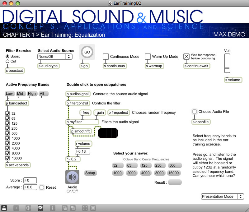
The icon shown in Figure 1.61 indicates there are supplements available that use the Max software. Max (formerly called Max/MSP/Jitter) is a real-time graphical programming environment for music, audio, and other media developed by Cycling ‘74. The core program, Max, provides the user interface, MIDI objects, timing for event-driven programming, and inter-object communications. This functionality is extended with the MSP and Jitter modules. MSP supports real-time audio synthesis and digital signal processing. Jitter adds the ability to work with video. Max programs, called patchers, can be easily distributed and run by anyone who downloads the free Max runtime program. The runtime allows you to open the patchers and interact with them. If you want to be able to make your own patchers or make changes to existing ones, you need to purchase the full version. Max can also compile patchers into executable applications. In this book, Max demos are finished patchers that demonstrate a concept. Max programming exercises are projects that ask you to create or modify your own patcher from a given set of requirements. We provide example solutions for Max programming exercises in the solutions section of our website.
Max is powerful enough to be useful in real-world theatre, performance, music, and even video gaming productions, allowing sound designers to create sound systems and functionality not available in off-the-shelf software. On the Cycling ’74 web page, you can find a list of interesting and creative applications.
Our Max demos require the Max runtime system and are optimized for Max version 6, which can be downloaded free at the Cycling ’74 website. Purchasing the full program is recommended for those who want to experiment with the demos more deeply or who want to complete the programming exercises. Figure 1.62 shows a series of Max patcher windows.
If you can’t afford Max, you might consider a free alternative, Pure Data, created by one of the originators of Max. Pure Data is open source software similar to Max in functionality and interface. For the Max programming exercises that involve audio programming, you might be able to use Pure Data and save yourself some money. However, PureData’s documentation is not nearly as comprehensive as the documentation for Max.
1.6.4 MATLAB and Octave

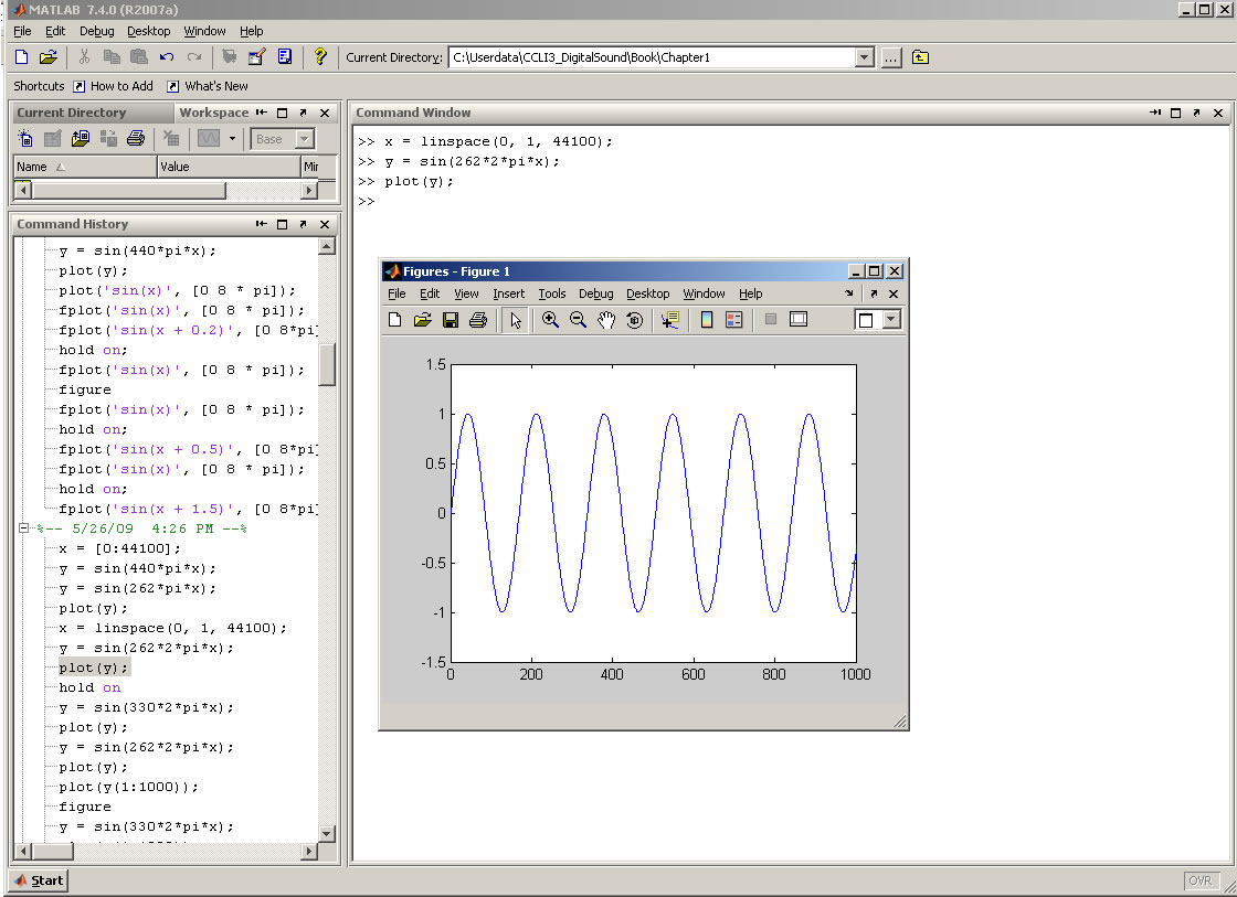
The icon shown in Figure 1.63 indicates there is a MATLAB exercise available for that section of the book. MATLAB (Figure 1.64) is a commercial mathematical modeling tool that allows you to experiment with digital sound at a low level of abstraction. MATLAB, which stands for “matrix lab,” is adept at manipulating matrices and arrays of data. Essentially, matrices are tables of information, and arrays are lists. Digital audio data related to a sound or piece of music is nothing more than an array of audio samples. The audio samples are generated in one of two basic ways in MATLAB. Sound can be recorded in an audio processing program like Adobe Audition, saved as an uncompressed PCM or a WAV file, and then input into MATLAB. Alternatively, it can be generated directly in MATLAB through the execution of sine functions. A sine function is given a frequency and amplitude related to the pitch and loudness of the desired sound. Executing a sine function at evenly spaced points produces numbers that constitute the audio data. Sine functions also can be added to each other to create complex sounds, the sound data can be plotted on a graph, and the sounds can be played in MATLAB. Operations on sine functions lay bare the mathematics of audio processing to give you a deeper understanding of filters, special effects, quantization error, dithering, and the like. Although such operations are embedded at a high level of abstraction in tools like Logic and Audition, MATLAB allows you to create them “by hand” so that you really understand how they work.
MATLAB also has extra toolkits that provide higher-level functions. For example, the signal processing toolkit gives you access to functions such as specialized waveform generators, transforms, frequency responses, impulse responses, FIR filters, IIR filters, and zero-pole diagram manipulations. The associated graphs help you to visualize how sound is changed when mathematical operations alter the properties of sound, amplitude, and phase.
GNU Octave is an open source alternative to MATLAB that runs under the Linux, Unix, Mac OS X, or Windows operating systems. Like MATLAB, its specialty is array operations. Octave has most of the basic functionality of MATLAB, including the ability to read in or generate audio data, plot the data, perform basic array-based operations like adding or multiplying sine functions, and handle complex numbers. Octave doesn’t have the extensive signal processing toolbox that MATLAB offers. However, third-party extensions to Octave are freely downloadable on the web, and at least one third-party signal processing toolkit has been developed with filtering, windowing, and display functions.
1.6.5 C++ and Java Programming Exercises

[aside]Because the audio processing implemented in these exercises is done at a fairly low level of abstraction, the solutions we provide for the C++ programming exercises are written primarily in C, without emphasis on the object-oriented features of C++. For convenience, we use a few C++ constructs like dynamic memory allocation with new and variable declarations anywhere in the program.[/aside]
This book is intended to be useful not only to musicians, digital sound designers, and sound engineers, but also to computer scientists specializing in digital sound. Thus we include examples of sound processing done at a low level of abstraction, through C++ programs (Figure 1.65). The C++ programs that we use as examples are done on the Linux operating system. Linux is a good platform for audio programming because it is open-source, allowing you to have direct access to the sound card and operating system. Windows, in contrast, is much more of a black box. Thus, low-level sound programming is harder to do in this environment.
If you have access to a computer running under Linux, you probably already have a C++ compiler installed. If not, you can download and install a GNU compiler. You can also try our examples under Unix, a relative of Linux. Your computer and operating system dictate what header files need to be included in your programs, so you may need to check the documentation on this.
Some Java programming exercises are also included with this book. Java allows you to handle sound at a higher level of abstraction with packages such as java.sound.sampled and java.sound.midi. You’ll need a Java compiler and run-time to work with these programs.
1.7 Where to Go from Here
We’ve included lot of information in this section. Don’t worry if you don’t completely understand everything yet. As you go through each chapter, you’ll have the opportunity to experiment with all of these tools until you become confident with them. For now, start building up your workstation with the tools we’ve suggested, and enjoy the ride.
1.8 References
Franz, David. Recording and Producing in the Home Studio: A Complete Guide. Boston, MA: Berklee Press, 2004.
Kirn, Peter. Digital Audio: Industrial-Strength Production Techniques. Berkeley, CA: Peachpit Press, 2006.
Pohlmann, Ken C. The Compact Disc Handbook. Middleton, WI: A-R Editions, Inc., 1992.
Toole, Betty A. Ada, The Enchantress of Numbers. Mill Valley, CA: Strawberry Press, 1992.
2.1.1 Sound Waves, Sine Waves, and Harmonic Motion
Working with digital sound begins with an understanding of sound as a physical phenomenon. The sounds we hear are the result of vibrations of objects – for example, the human vocal chords, or the metal strings and wooden body of a guitar. In general, without the influence of a specific sound vibration, air molecules move around randomly. A vibrating object pushes against the randomly-moving air molecules in the vicinity of the vibrating object, causing them first to crowd together and then to move apart. The alternate crowding together and moving apart of these molecules in turn affects the surrounding air pressure. The air pressure around the vibrating object rises and falls in a regular pattern, and this fluctuation of air pressure, propagated outward, is what we hear as sound.
Sound is often referred to as a wave, but we need to be careful with the commonly-used term “sound wave,” as it can lead to a misconception about the nature of sound as a physical phenomenon. On the one hand, there’s the physical wave of energy passed through a medium as sound travels from its source to a listener. (We’ll assume for simplicity that the sound is traveling through air, although it can travel through other media.) Related to this is the graphical view of sound, a plot of air pressure amplitude at a particular position in space as it changes over time. For single-frequency sounds, this graph takes the shape of a “wave,” as shown in Figure 2.1. More precisely, a single-frequency sound can be expressed as a sine function and graphed as a sine wave (as we’ll describe in more detail later). Let’s see how these two things are related.
[wpfilebase tag=file id=105 tpl=supplement /]
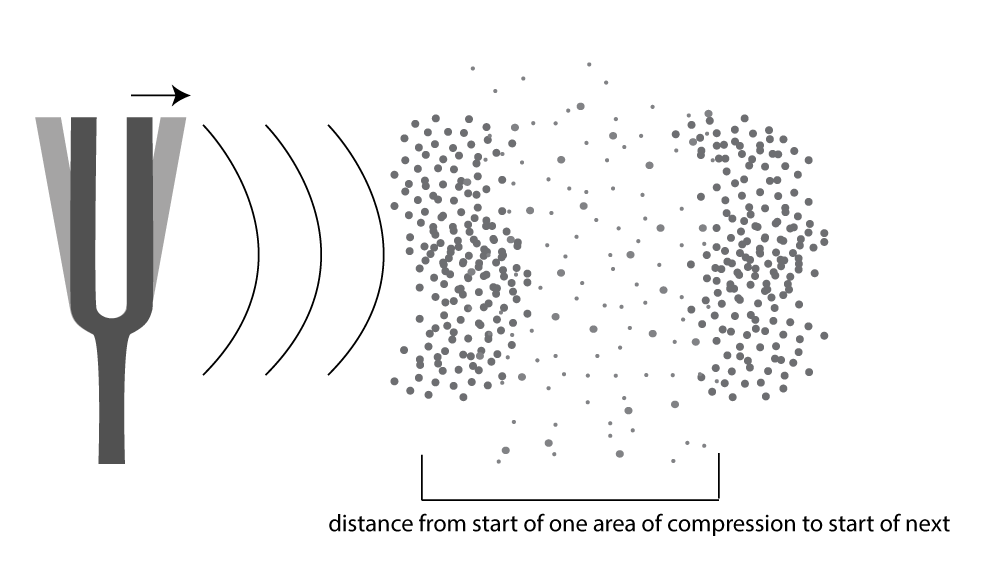
First, consider a very simple vibrating object – a tuning fork. When the tuning fork is struck, it begins to move back and forth. As the prong of the tuning fork vibrates outward (in Figure 2.2), it pushes the air molecules right next to it, which results in a rise in air pressure corresponding to a local increase in air density. This is called compression. Now, consider what happens when the prong vibrates inward. The air molecules have more room to spread out again, so the air pressure beside the tuning fork falls. The spreading out of the molecules is called decompression or rarefaction. A wave of rising and falling air pressure is transmitted to the listener’s ear. This is the physical phenomenon of sound, the actual sound wave.
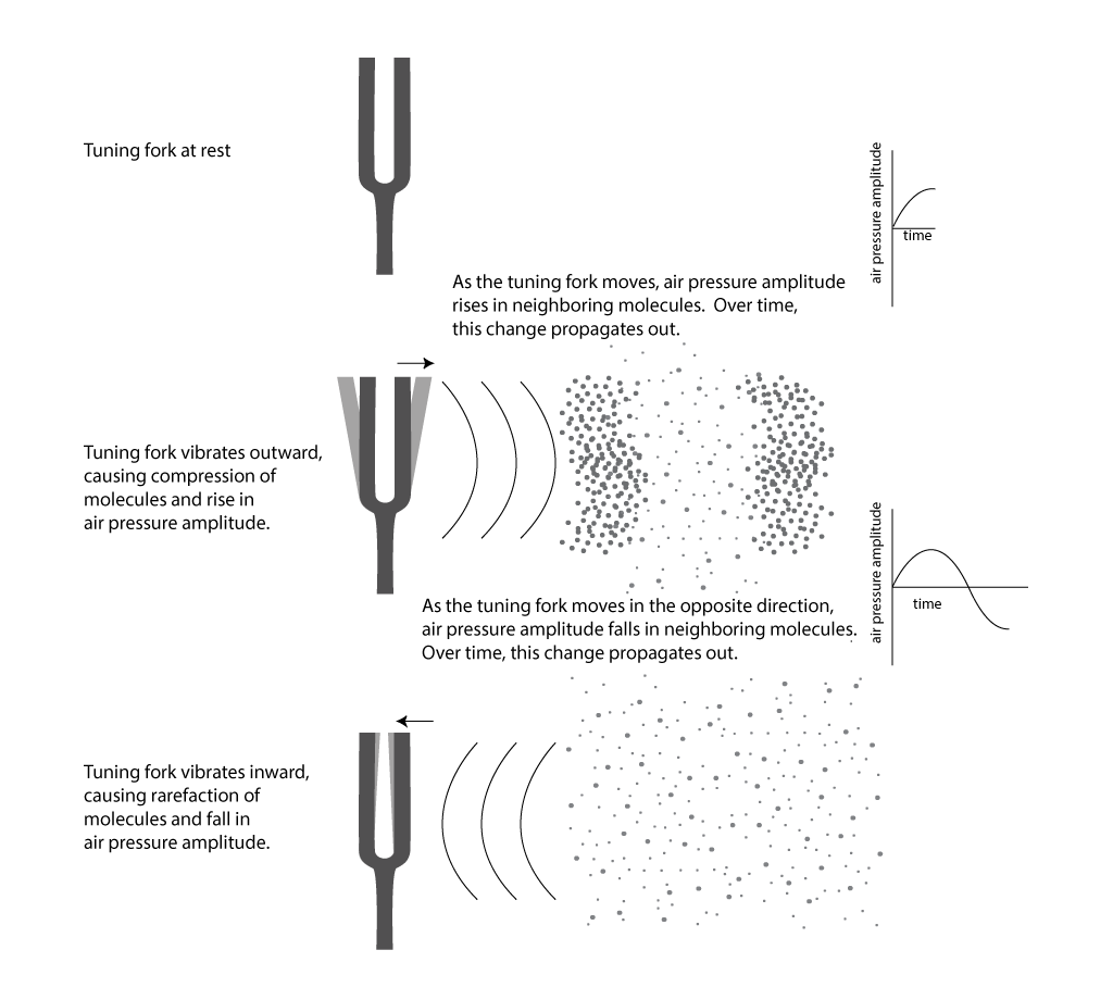
Assume that a tuning fork creates a single-frequency wave. Such a sound wave can be graphed as a sine wave, as illustrated in Figure 2.1. An incorrect understanding of this graph would be to picture air molecules going up and down as they travel across space from the place in which the sound originates to the place in which it is heard. This would be as if a particular molecule starts out where the sound originates and ends up in the listener’s ear. This is not what is being pictured in a graph of a sound wave. It is the energy, not the air molecules themselves, that is being transmitted from the source of a sound to the listener’s ear. If the wave in Figure 2.1 is intended to depict a single-frequency sound wave, then the graph has time on the x-axis (the horizontal axis) and air pressure amplitude on the y-axis. As described above, the air pressure rises and falls. For a single-frequency sound wave, the rate at which it does this is regular and continuous, taking the shape of a sine wave.
Thus, the graph of a sound wave is a simple sine wave only if the sound has only one frequency component in it – that is, just one pitch. Most sounds are composed of multiple frequency components – multiple pitches. A sound with multiple frequency components also can be represented as a graph which plots amplitude over time; it’s just a graph with a more complicated shape. For simplicity, we sometimes use the term “sound wave” rather than “graph of a sound wave” for such graphs, assuming that you understand the difference between the physical phenomenon and the graph representing it.
The regular pattern of compression and rarefaction described above is an example of harmonic motion, also called harmonic oscillation. Another example of harmonic motion is a spring dangling vertically. If you pull on the bottom of the spring, it will bounce up and down in a regular pattern. Its position – that is, its displacement from its natural resting position – can be graphed over time in the same way that a sound wave’s air pressure amplitude can be graphed over time. The spring’s position increases as the spring stretches downward, and it goes to negative values as it bounces upwards. The speed of the spring’s motion slows down as it reaches its maximum extension, and then it speeds up again as it bounces upwards. This slowing down and speeding up as the spring bounces up and down can be modeled by the curve of a sine wave. In the ideal model, with no friction, the bouncing would go on forever. In reality, however, friction causes a damping effect such that the spring eventually comes to rest. We’ll discuss damping more in a later chapter.
Now consider how sound travels from one location to another. The first molecules bump into the molecules beside them, and they bump into the next ones, and so forth as time goes on. It’s something like a chain reaction of cars bumping into one another in a pile-up wreck. They don’t all hit each other simultaneously. The first hits the second, the second hits the third, and so on. In the case of sound waves, this passing along of the change in air pressure is called sound wave propagation. The movement of the air molecules is different from the chain reaction pile up of cars, however, in that the molecules vibrate back and forth. When the molecules vibrate in the direction opposite of their original direction, the drop in air pressure amplitude is propagated through space in the same way that the increase was propagated.
Be careful not to confuse the speed at which a sound wave propagates and the rate at which the air pressure amplitude changes from highest to lowest. The speed at which the sound is transmitted from the source of the sound to the listener of the sound is the speed of sound. The rate at which the air pressure changes at a given point in space – i.e., vibrates back and forth – is the frequency of the sound wave. You may understand this better through the following analogy. Imagine that you’re watching someone turn a flashlight on and off, repeatedly, at a certain fixed rate in order to communicate a sequence of numbers to you in binary code. The image of this person is transmitted to your eyes at the speed of light, analogous to the speed of sound. The rate at which the person is turning the flashlight on and off is the frequency of the communication, analogous to the frequency of a sound wave.
The above description of a sound wave implies that there must be a medium through which the changing pressure propagates. We’ve described sound traveling through air, but sound also can travel through liquids and solids. The speed at which the change in pressure propagates is the speed of sound. The speed of sound is different depending upon the medium in which sound is transmitted. It also varies by temperature and density. The speed of sound in air is approximately 1130 ft/s (or 344 m/s). Table 2.1 shows the approximate speed in other media.
[table caption=”Table 2.1 The Speed of sound in various media” colalign=”center|center|center” width=”80%”]
Medium,Speed of sound in m/s, Speed of sound in ft/s
“air (20° C, which is 68° F)”,344,”1,130″
“water (just above 0° C, which is 32° F)”,”1,410″,”4,626″
steel,”5,100″,”16,700″
lead,”1,210″,”3,970″
glass,”approximately 4,000~~(depending on type of glass)”,”approximately 13,200″
[/table]
[aside width=”75px”]
feet = ft
seconds = s
meters = m
[/aside]
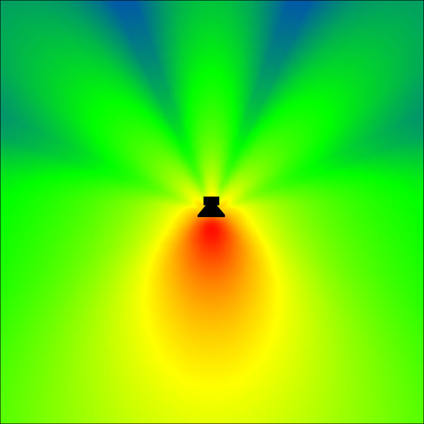
For clarity, we’ve thus far simplified the picture of how sound propagates. Figure 2.2 makes it look as though there’s a single line of sound going straight out from the tuning fork and arriving at the listener’s ear. In fact, sound radiates out from a source at all angles in a sphere. Figure 2.3 shows a top-view image of a real sound radiation pattern, generated by software that uses sound dispersion data, measured from an actual loudspeaker, to predict how sound will propagate in a given three-dimensional space. In this case, we’re looking at the horizontal dispersion of the loudspeaker. Colors are used to indicate the amplitude of sound, going highest to lowest from red to yellow to green to blue. The figure shows that the amplitude of the sound is highest in front of the loudspeaker and lowest behind it. The simplification in Figure 2.2 suffices to give you a basic concept of sound as it emanates from a source and arrives at your ear. Later, when we begin to talk about acoustics, we’ll consider a more complete picture of sound waves.
Sound waves are passed through the ear canal to the eardrum, causing vibrations which pass to little hairs in the inner ear. These hairs are connected to the auditory nerve, which sends the signal onto the brain. The rate of a sound vibration – its frequency – is perceived as its pitch by the brain. The graph of a sound wave represents the changes in air pressure over time resulting from a vibrating source. To understand this better, let’s look more closely at the concept of frequency and other properties of sine waves.
2.1.2 Properties of Sine Waves
We assume that you have some familiarity with sine waves from trigonometry, but even if you don’t, you should be able to understand some basic concepts of this explanation.
A sine wave is a graph of a sine function . In the graph, the x-axis is the horizontal axis, and the y-axis is the vertical axis. A graph or phenomenon that takes the shape of a sine wave – oscillating up and down in a regular, continuous manner – is called a sinusoid.
In order to have the proper terminology to discuss sound waves and the corresponding sine functions, we need to take a little side trip into mathematics. We’ll first give the sine function as it applies to sound, and then we’ll explain the related terminology.
[equation caption=”Equation 2.1″]A single-frequency sound wave with frequency f , maximum amplitude A, and phase θ is represented by the sine function
$$!y=A\sin \left ( 2\pi fx+\theta \right )$$
where x is time and y is the amplitude of the sound wave at time x.[/equation]
[wpfilebase tag=file id=106 tpl=supplement /]
Single-frequency sound waves are sinusoidal waves. Although pure single-frequency sound waves do not occur naturally, they can be created artificially by means of a computer. Naturally occurring sound waves are combinations of frequency components, as we’ll discuss later in this chapter.
The graph of a sound wave is repeated Figure 2.4 with some of its parts labeled. The amplitude of a wave is its y value at some moment in time given by x. If we’re talking about a pure sine wave, then the wave’s amplitude, A, is the highest y value of the wave. We call this highest value the crest of the wave. The lowest value of the wave is called the trough. When we speak of the amplitude of the sine wave related to sound, we’re referring essentially to the change in air pressure caused by the vibrations that created the sound. This air pressure, which changes over time, can be measured in Newtons/meter2 or, more customarily, in decibels (abbreviated dB), a logarithmic unit explained in detail in Chapter 4. Amplitude is related to perceived loudness. The higher the amplitude of a sound wave, the louder it seems to the human ear.
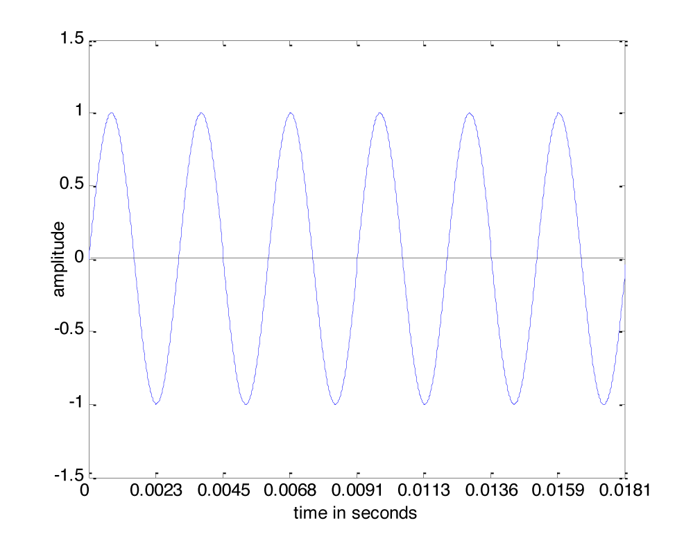
In order to define frequency, we must first define a cycle. A cycle of a sine wave is a section of the wave from some starting position to the first moment at which it returns to that same position after having gone through its maximum and minimum amplitudes. Usually, we choose the starting position to be at some position where the wave crosses the x-axis, or zero crossing, so the cycle would be from that position to the next zero crossing where the wave starts to repeat, as shown in Figure 2.4.
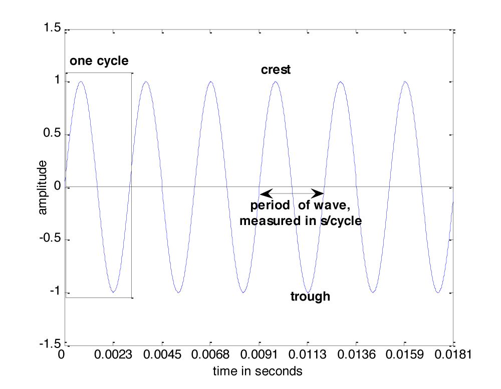
The frequency of a wave, f, is the number of cycles per unit time, customarily the number of cycles per second. A unit that is used in speaking of sound frequency is Hertz, defined as 1 cycle/second, and abbreviated Hz. In Figure 2.4, the time units on the x-axis are seconds. Thus, the frequency of the wave is 6 cycles/0.0181 seconds » 331 Hz. Henceforth, we’ll use the abbreviation s for seconds and ms for milliseconds.
Frequency is related to pitch in human perception. A single-frequency sound is perceived as a single pitch. For example, a sound wave of 440 Hz sounds like the note A on a piano (just above middle C). Humans hear in a frequency range of approximately 20 Hz to 20,000 Hz. The frequency ranges of most musical instruments fall between about 50 Hz and 5000 Hz. The range of frequencies that an individual can hear varies with age and other individual factors.
The period of a wave, T, is the time it takes for the wave to complete one cycle, measured in s/cycle. Frequency and period have an inverse relationship, given below.
[equation caption=”Equation 2.2″]Let the frequency of a sine wave be and f the period of a sine wave be T. Then
$$!f=1/T$$
and
$$!T=1/f$$
[/equation]
The period of the wave in Figure 2.4 is about three milliseconds per cycle. A 440 Hz wave (which has a frequency of 440 cycles/s) has a period of 1 s/440 cycles, which is about 0.00227 s/cycle. There are contexts in which it is more convenient to speak of period only in units of time, and in these contexts the “per cycle” can be omitted as long as units are handled consistently for a particular computation. With this in mind, a 440 Hz wave would simply be said to have a period of 2.27 milliseconds.
[wpfilebase tag=file id=28 tpl=supplement /]
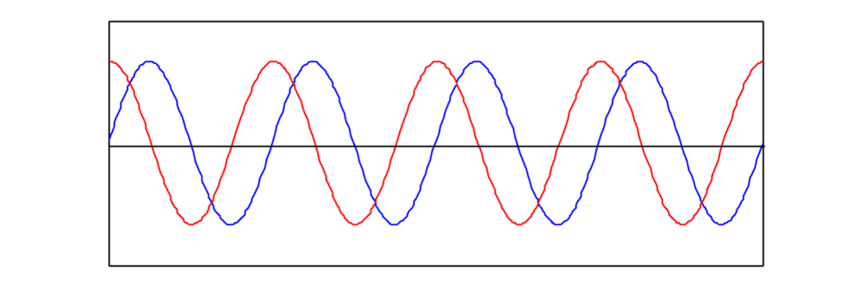
The phase of a wave, θ, is its offset from some specified starting position at x = 0. The sine of 0 is 0, so the blue graph in Figure 2.5 represents a sine function with no phase offset. However, consider a second sine wave with exactly the same frequency and amplitude, but displaced in the positive or negative direction on the x-axis relative to the first, as shown in Figure 2.5. The extent to which two waves have a phase offset relative to each other can be measured in degrees. If one sine wave is offset a full cycle from another, it has a 360 degree offset (denoted 360o); if it is offset a half cycle, is has a 180 o offset; if it is offset a quarter cycle, it has a 90 o offset, and so forth. In Figure 2.5, the red wave has a 90 o offset from the blue. Equivalently, you could say it has a 270 o offset, depending on whether you assume it is offset in the positive or negative x direction.
Wavelength, λ, is the distance that a single-frequency wave propagates in space as it completes one cycle. Another way to say this is that wavelength is the distance between a place where the air pressure is at its maximum and a neighboring place where it is at its maximum. Distance is not represented on the graph of a sound wave, so we cannot directly observe the wavelength on such a graph. Instead, we have to consider the relationship between the speed of sound and a particular sound wave’s period. Assume that the speed of sound is 1130 ft/s. If a 440 Hz wave takes 2.27 milliseconds to complete a cycle, then the position of maximum air pressure travels 1 cycle * 0.00227 s/cycle * 1130 ft/s in one wavelength, which is 2.57 ft. This relationship is given more generally in the equation below.
[equation caption=”Equation 2.3″]Let the frequency of a sine wave representing a sound be f, the period be T, the wavelength be λ, and the speed of sound be c. Then
$$!\lambda =cT$$
or equivalently
$$!\lambda =c/f$$
[/equation]
2.1.5 Digitizing Sound Waves
In this chapter, we have been describing sound as continuous changes of air pressure amplitude. In this sense, sound is an analog phenomenon – a physical phenomenon that could be represented as continuously changing voltages. Computers require that we use a discrete representation of sound. In particular, when sound is captured as data in a computer, it is represented as a list of numbers. Capturing sound in a form that can be handled by a computer is a process called analog-to-digital conversion, whereby the amplitude of a sound wave is measured at evenly-spaced intervals in time – typically 44,100 times per second, or even more. Details of analog-to-digital conversion are covered in Chapter 5. For now, it suffices to think of digitized sound as a list of numbers. Once a computer has captured sound as a list of numbers, a whole host of mathematical operations can be performed on the sound to change its loudness, pitch, frequency balance, and so forth. We’ll begin to see how this works in the following sections.