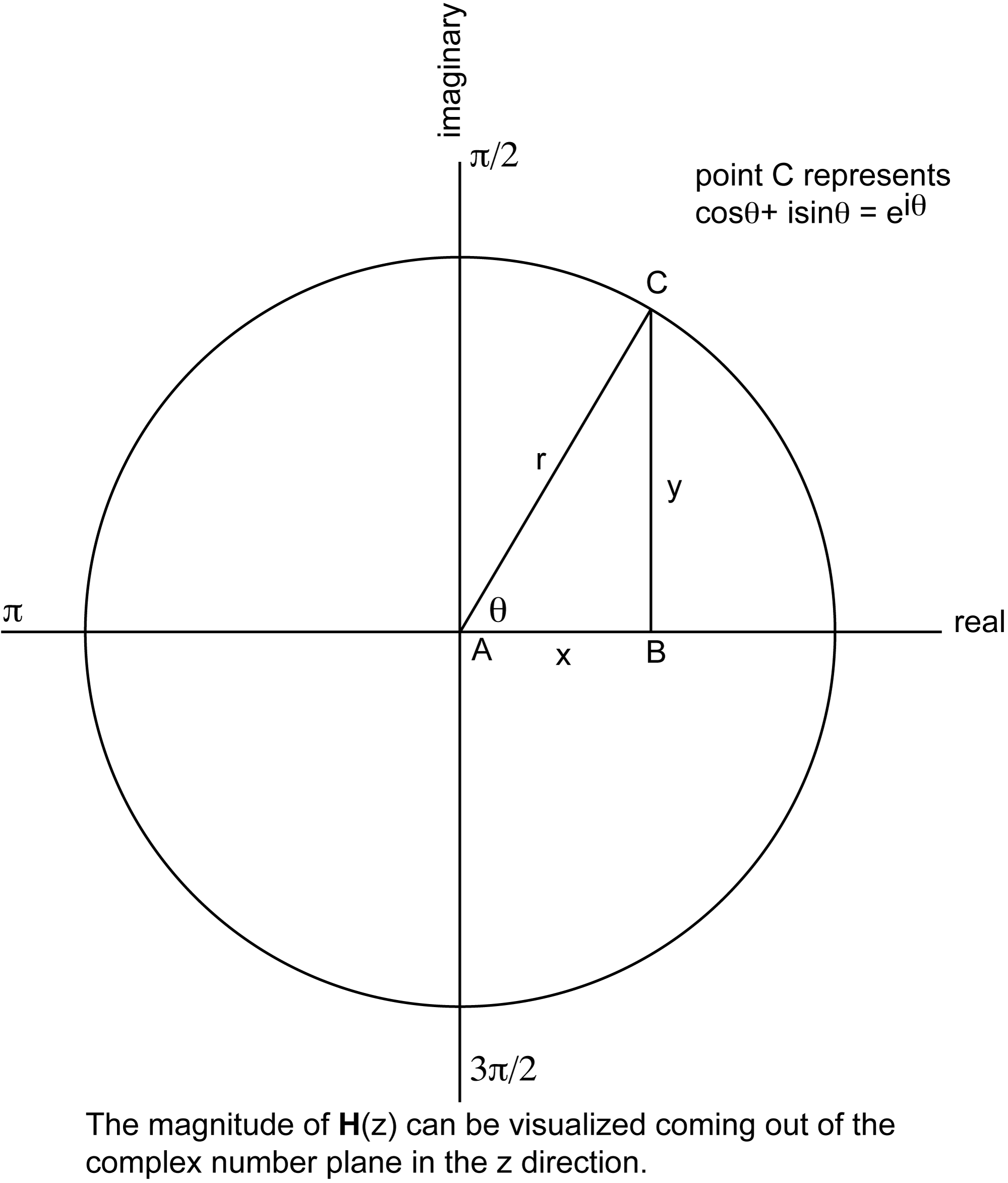
The function $$\mathbf{H}\left ( z \right )$$ defining a filter has a complex number z as its input parameter. Complex numbers are expressed as $$a+bi$$, where a is the real number component, b is the coefficient of the imaginary component, and i is $$\sqrt{-1}$$. The complex number plane can be graphed as shown in Figure 7.37, with the real component on the horizontal axis and the coefficient of the imaginary component on the vertical axis. Let’s look at how this works.

With regard to Figure 7.37, let x, y, and r denote the lengths of line segments $$\overline{AB}$$, $$\overline{BC}$$, and $$\overline{AC}$$ , respectively. Since the circle is a unit circle, $$r=1$$. From trigonometric relations, we get

$$!x=\cos \theta$$

$$!y=\sin \theta$$

Point C represents the number $$\cos \theta +i\sin \theta$$ on the complex number plane. By Euler’s identity, $$\cos \theta +i\sin \theta=e^{i\theta }$$.  $$\mathbf{H}\left ( z \right )$$ is a function that is evaluated around the unit circle and graphed on the complex number plane. Since we are working with discrete values, we are evaluating the filter’s response at N discrete points evenly distributed around the unit circle. Specifically, the response for the $$k^{th}$$ frequency component is found by evaluating $$\mathbf{H}\left ( z_{k} \right )$$ at $$z=e^{i\theta }=e^{i\frac{2\pi k}{N}}$$ where N is the number of frequency components. The output,  $$\mathbf{H}\left ( z_{k} \right )$$, is a complex number, but if you want to picture the output in the graph, you can consider only the magnitude of $$\mathbf{H}\left ( z_{k} \right )$$, which would be a real number coming out of the complex number plane (as we’ll show in Figure 7.41). This helps you to visualize how the filter attenuates or boosts the magnitudes of different frequency components.

This leads us to a description of the zero-pole diagram, a graph of a filter’s transfer function that marks places where the filter does the most or least attenuation (the zeroes and poles, as shown in Figure 7.38). As the numerator of $$\frac{\mathbf{Y}\left ( z \right )}{\mathbf{X}\left ( z \right )}$$ goes to 0, the output frequency is getting smaller relative to the input frequency. This is called a zero. As the denominator goes to 0, the output frequency is getting larger relative to the input frequency. This is called a pole.

To see the behavior of the filter, we can move around the unit circle looking at each frequency component at point $$e^{i\theta }$$ where $$\theta =\frac{2\pi k}{N}$$ for $$0\leq k< N-1$$. Let $$d_{zero}$$ be the point’s distance from a zero and $$d_{pole}$$ be the point’s distance from a pole. If, as you move from point $$P_{k}$$ to point $$P_{k+1}$$ (these points representing input frequencies $$e^{i\frac{2\pi k}{N}}$$ and $$e^{i\frac{2\pi\left ( k+1 \right )}{N}}$$ respectively), the ratio $$\frac{d_{zero}}{d_{pole}}$$ gets larger, then the filter is progressively allowing more of the frequency $$e^{i\frac{2\pi k}{N}}$$ to “pass through” as opposed to $$e^{i\frac{2\pi\left ( k+1 \right )}{N}}$$.

Let’s try this mathematically with a couple of examples. These examples will get you started in your understanding of zero-pole diagrams and the graphing of filters, but the subject is complex. MATLAB’s Help has more examples and more explanations, and you can find more details in the books on digital signal processing listed in our references.

First let’s try a simple FIR filter. The coefficients for this filter are . In the time domain, this filter can be seen as a convolution represented as follows:

[equation caption=”Equation 7.11 Convolution for a simple filter in the time domain”]

$$!\mathbf{y}\left ( n \right )=\sum_{k=0}^{1}\mathbf{h}\left ( k \right )\mathbf{x}\left ( n-k \right )=\mathbf{x}\left ( n \right )-0.5\mathbf{x}\left ( n-1 \right )$$

[/equation]

Converting the filter to the frequency domain by the z-transform, we get

[equation caption=”Equation 7.12 Delay filter represented as a transfer function”]

$$!\mathbf{H}\left ( z \right )=1-0.5z^{-1}=\frac{z\left ( 1-0.5z^{-1} \right )}{z}=\frac{z-0.5}{z}$$

[/equation]

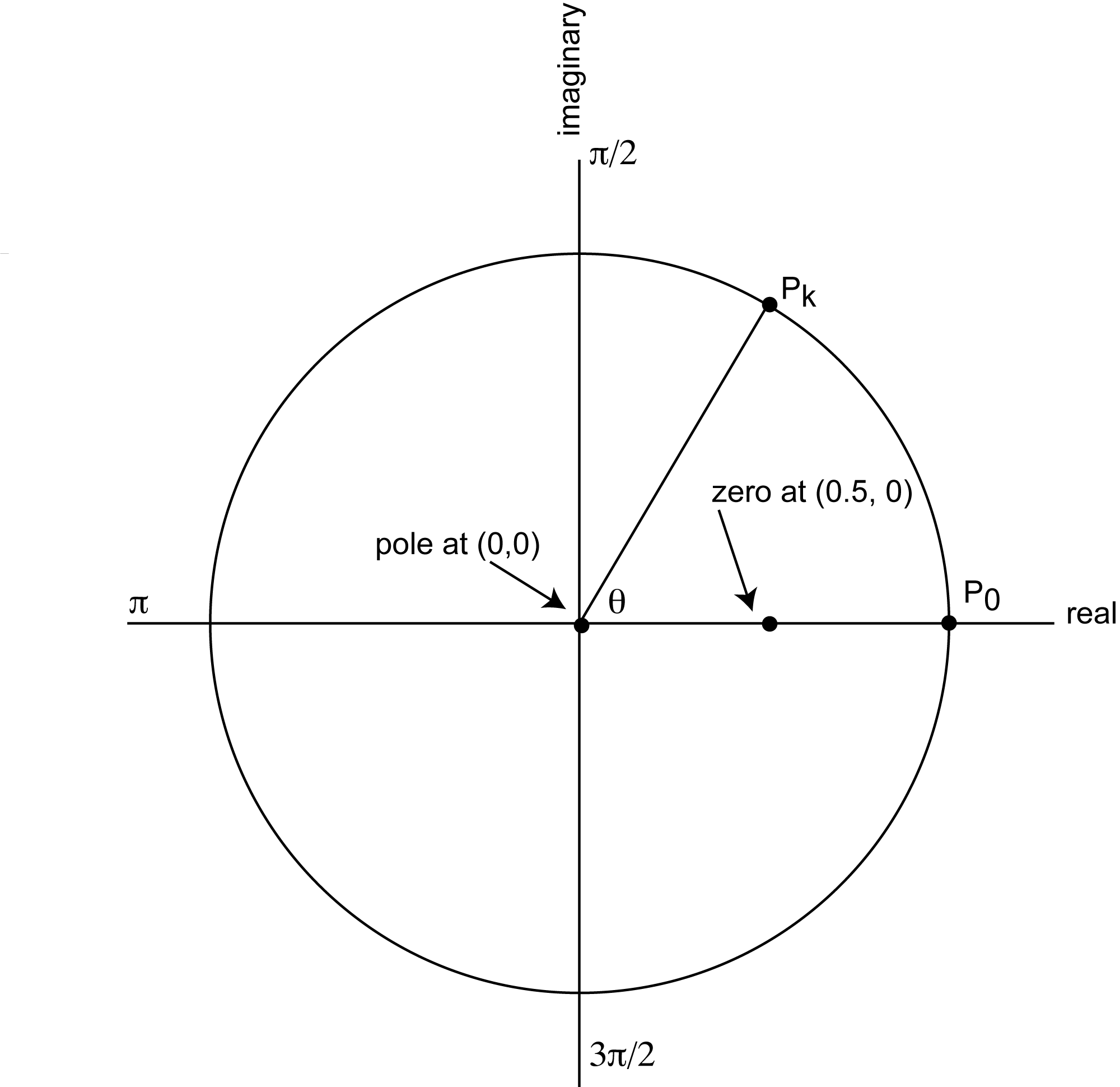
In the case of this simple filter, it’s easy to see where the zeroes and poles are. At $$z=0.5$$, the numerator is 0. Thus, a zero is at point (0.5, 0). At z = 0, the denominator is 0. Thus, a pole is at (0,0). There is no imaginary component to either the zero or the pole, so the coefficient of the imaginary part of the complex number is 0 in both cases.

Once we have the zeroes and poles, we can plot them on the graph representing the filter, $$\mathbf{H}\left ( z \right )$$, as shown in Figure 7.38. To analyze the filter’s effect on frequency components, consider the $$k^{th}$$ discrete point on the unit circle, point $$P_{k}$$, and the behavior of filter $$\mathbf{H}\left ( z \right )$$ at that point. Point $$P_{0}$$ is at the origin, and the angle formed between the x-axis and the line between $$P_{0}$$ and $$P_{k}$$is $$\theta =\frac{2\pi k}{N}$$. Each such point $$P_{k}$$ at angle $$\theta =\frac{2\pi k}{N}$$ corresponds to a frequency component $$e^{i}\frac{2\pi k}{N}$$ in the audio that is being filtered. Assume that the Nyquist frequency has been normalized to $$\pi$$. Thus, by the Nyquist theorem, the only valid frequency components to consider are between 0 and $$\pi$$. Let $$d_{zero}$$ be the distance between $$P_{k}$$ and a zero of the filter, and let $$d_{pole}$$ be the distance between $$P_{k}$$ and a pole. The magnitude of the frequency response, $$\mathbf{H}\left ( z \right )$$, will be smaller in proportion to $$\frac{d_{zero}}{d_{pole}}$$. For this example, the pole is at the origin so for all points $$P_{k}$$, $$d_{pole}$$ is 1. Thus, the magnitude of $$\frac{d_{zero}}{d_{pole}}$$ depends entirely on $$d_{zero}$$. As $$d_{zero}$$ gets larger, the frequency response gets larger. $$d_{zero}$$ increases as you move from $$\theta =0$$ to $$\theta =\pi$$. Since the frequency response increases as frequency increases, this filter is a high-pass filter, attenuating low frequencies more than high ones.

Now let’s try a simple IIR filter. Say that the equation for the filter is this:

[equation caption=”Equation 7.13 Equation for an IIR filter”]

$$!\mathbf{y}\left ( n \right )=\mathbf{x}\left ( n \right )-\mathbf{x}\left ( n-2 \right )-0.49\mathbf{y}\left ( n-2 \right )$$

[/equation]

The coefficients for the forward filter are $$\left [ 1,0,-1\right ]$$, and the coefficients for the feedback filter are $$\left [ 0, -0.49\right ]$$. Applying the transfer function form of the filter, we get

[equation caption=”Equation 7.14 Equation for IIR filter, version 2″]

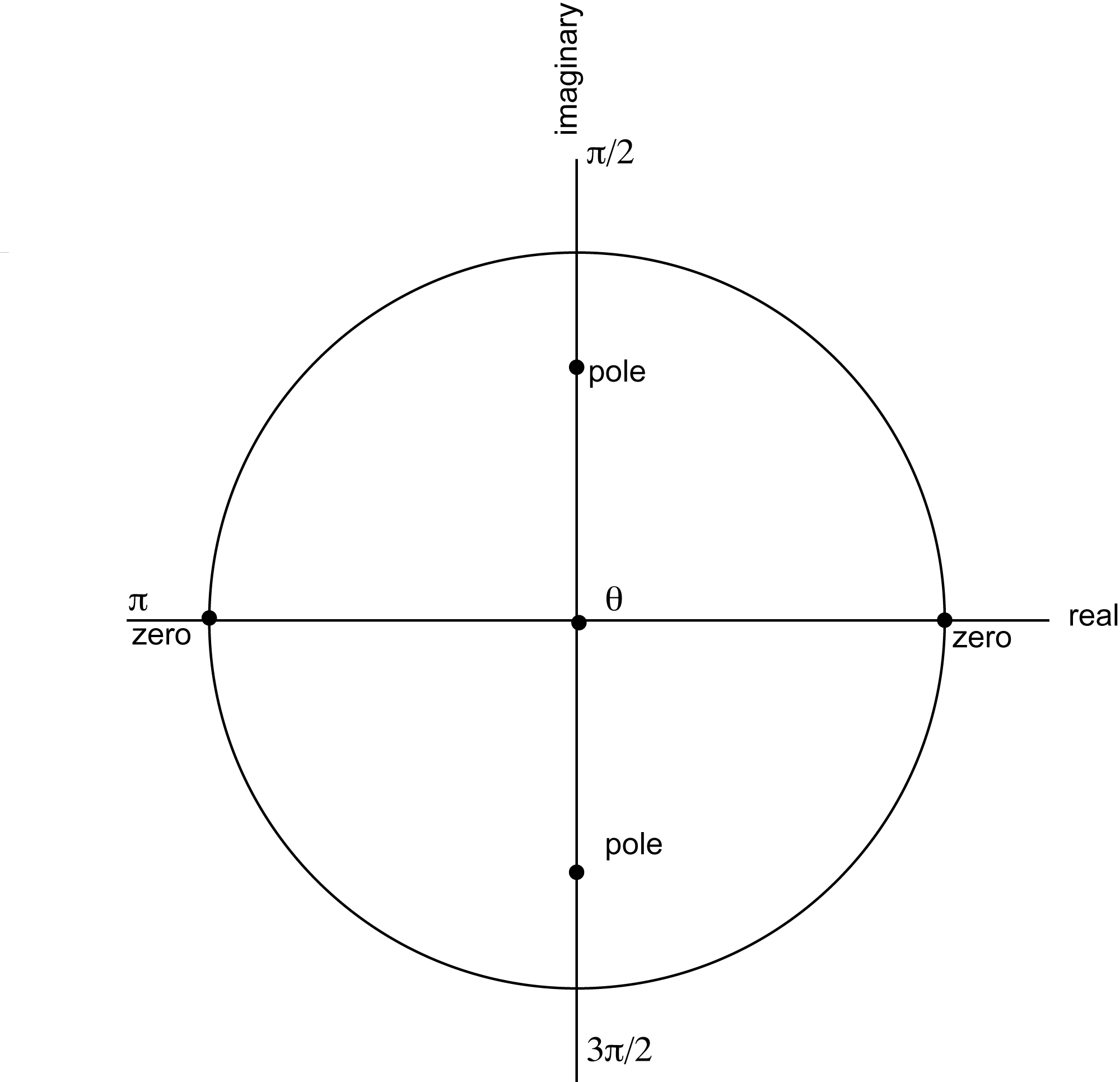
$$!\mathbf{H}\left ( z \right )=\frac{1-z^{-2}}{1-0.49z^{-2}}=\frac{z^{2}-1}{z^{2}-0.49}=\frac{\left ( z+1 \right )\left ( z-1 \right )}{\left ( z+0.7i \right )\left ( z-0.7i \right )}$$

[/equation]

From Equation 7.14, we can see that there are zeroes at $$z=1$$ and $$z=-1$$ and poles at $$z=0.7i$$ and $$z=-0.7i$$. The zeroes and poles are plotted in Figure 7.39. This diagram is harder to analyze by inspection because there are two zeroes and two poles.

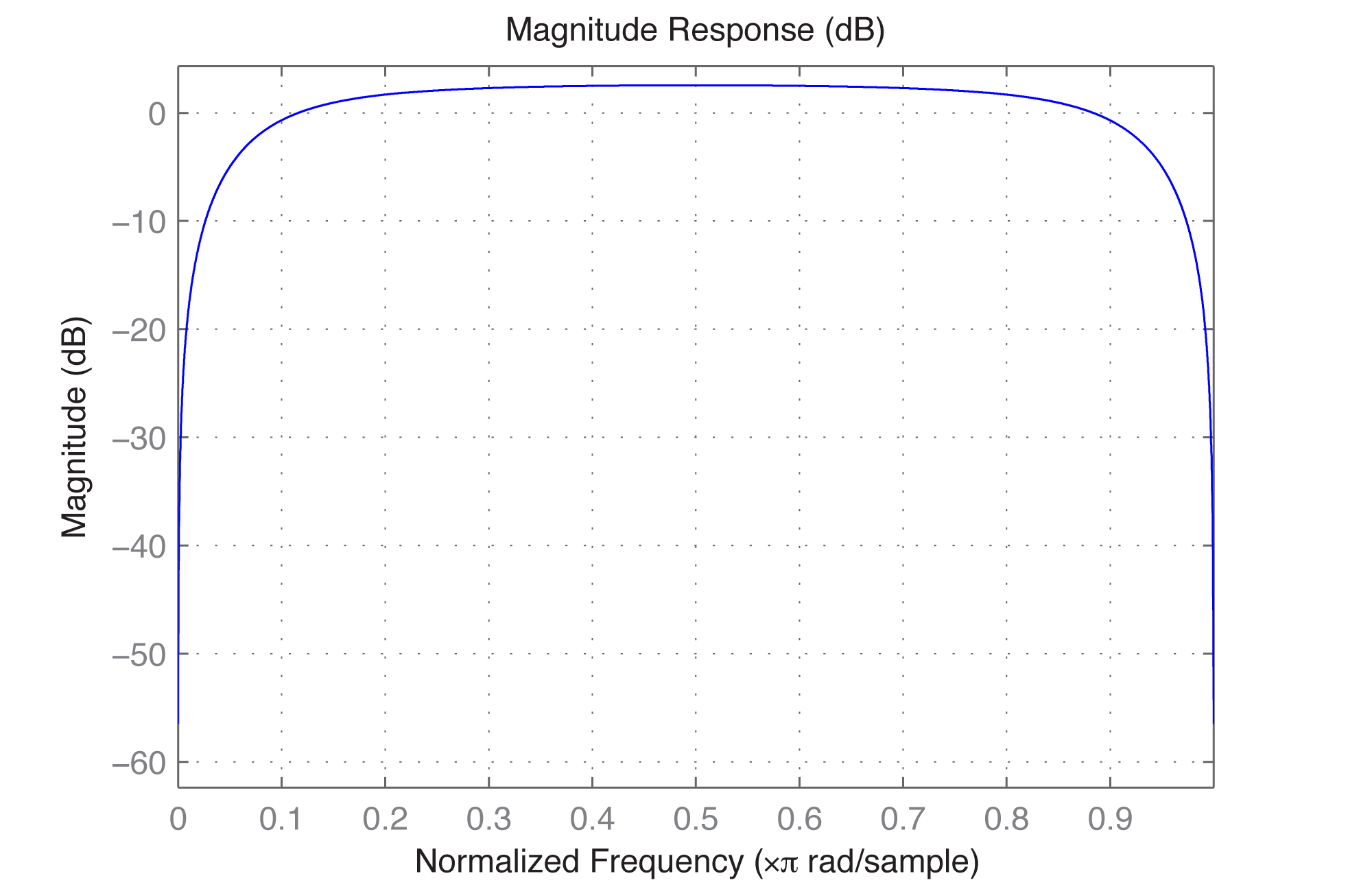
If we graph the frequency response of the filter, we can see that it’s a bandpass filter. We can do this with MATLAB’s fvtool (Filter Visualization Tool). The fvtool expects the coefficients of the transfer function (Equation 7.10) as arguments. The first argument of fvtool should be the coefficents of the numerator $$\left ( a_{0},a_{1},a_{2},\cdots \right )$$, and the second should be the coefficients of the denominator $$\left ( b_{1},b_{2},b_{3},\cdots \right )$$. Thus, the following MATLAB commands produce the graph of the frequency response, which shows that we have a bandpass filter with a rather wide band (Figure 7.40).

a = [1 0 -1];

b = [1 0 -0.49];

fvtool(a,b);

 

(You have to include the constant 1 as the first element of b.) MATLAB’s fvtool is discussed further in Section 7.3.9.

[wpfilebase tag=file id=167 tpl=supplement /]

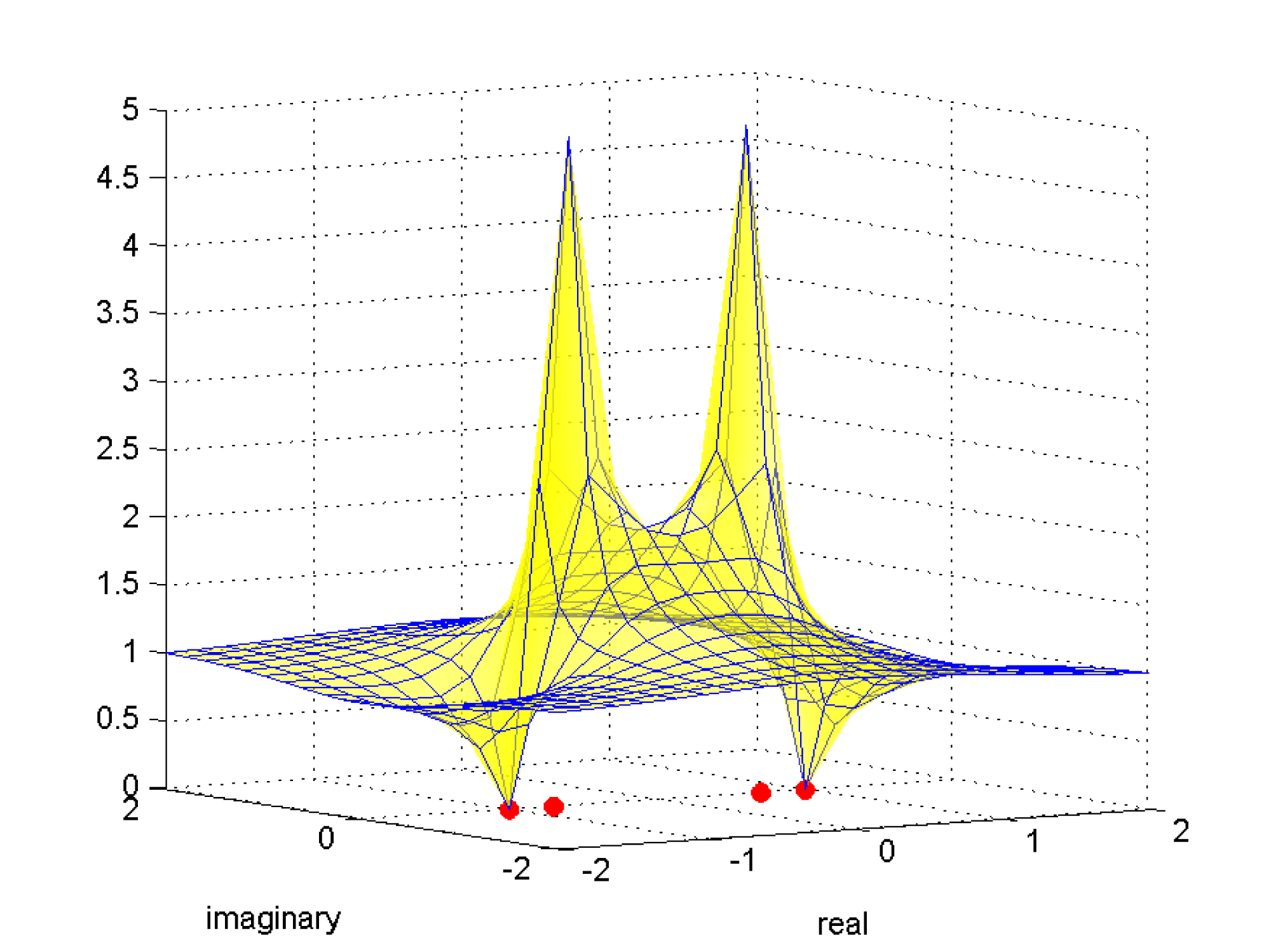
We can also graph the frequency response on the complex number plane, as we did with the zero-pole diagram, but this time we show the magnitude of the frequency response in the third dimension by means of a surface plot. This plot is shown in Figure 7.41. Writing a MATLAB function to create a graph such as this is left as an exercise.

In Chapter 4, we discussed comb filtering in the context of acoustics and showed how comb filters can be made by means of delays. Let’s review comb filtering now.

A comb filter is created when two identical copies of a sound are summed (in the air, by means of computer processing, etc.), with one copy being offset in time from the other. The amount of offset determines which frequencies are combed out. The equation that predicts the combed frequency is given below.

[equation caption=”Equation 7.15 Comb filtering”]

$$!\begin{matrix}\textrm{Given a delay of }t\textrm{ seconds between two identical copies of a sound, then the frequencies of }f_{i}\textrm{ that will be combed are }\\ f_{i}=\frac{2i+1}{2t}\textrm{ for all integers }i\geq 0\end{matrix}$$

[/equation]

For a sampling rate of 44.1 kHz, 0.01 is equivalent to 441 samples. This delay is demonstrated in the MATLAB code below, which applies a delay of 0.01 seconds to white noise and graphs the resulting frequencies. (The white noise was created in Audition and saved in a raw PCM file.)

fid = fopen('WhiteNoise.pcm', 'r');

y = fread(fid, 'int16');

y = y(1:44100);

first = y(442:44100);

second = y(1:441);

y2 = cat(1, first, second);

y3 = y + y2;

plot(abs(fft(y3)));

 

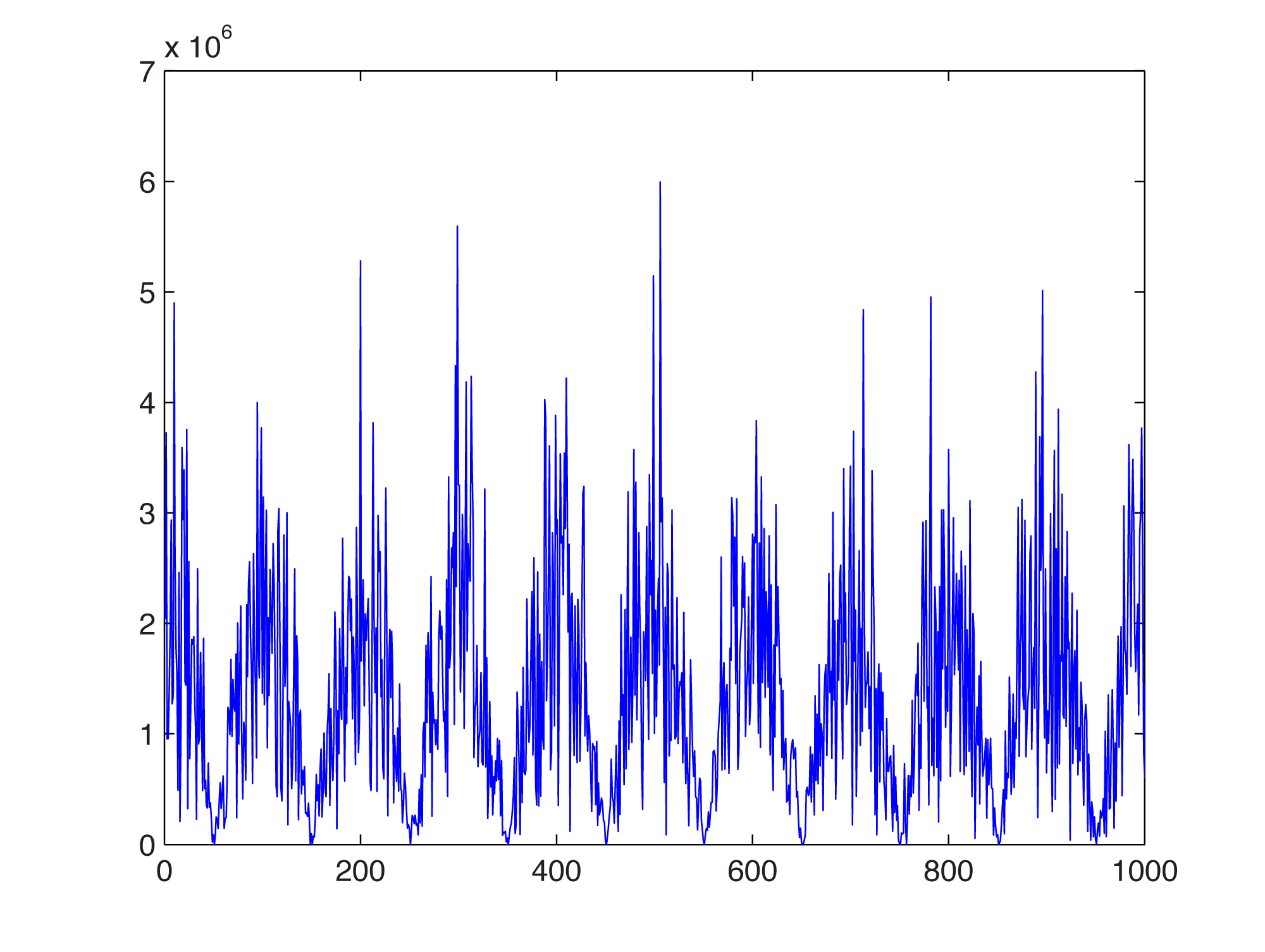
You can see in Figure 7.42 that with a delay of 0.01 seconds, the frequencies that are combed out are 50 Hz, 150 Hz, 250 Hz, and so forth, while frequencies of 100 Hz, 200 Hz, 300 Hz, and so forth are boosted.

We created the comb filter above “by hand” by shifting the sample values and summing them. We can also use MATLAB’s fvtool.

a = [1  zeroes(1,440) 0.5];

b = [1];

fvtool(a,b);

axis([0 .008 -8 6]);

 

The x-axis in Figure 7.43 is normalized to the Nyquist frequency. That is, for a sampling rate of 44.1 kHz, the Nyquist frequency of 22,050 Hz is normalized to 1. Thus, 50 Hz falls at position 0.002 and 100 Hz at about 0.0045, etc.

Comb filters can be expressed as either non-recursive FIR filters or recursive IIR filters. A simple non-recursive comb filter is expressed by the following equation:

[equation caption=”Equation 7.16 Equation for an FIR comb filter”]

$$!\begin{matrix}\mathbf{y}\left ( n \right )=\mathbf{x}\left ( n \right )+g \ast \mathbf{x}\left ( n-m \right )\\\textit{where }\mathbf{y}\textit{ is the filtered audio in the time domain}\\\mathbf{x}\textit{ is the original audio in the time domain}\\m\textit{ is the amount of delay in samples, and}\left | g \right |\leq 1\end{matrix}$$

[/equation]

In an FIR comb filter, a fraction of an earlier sample is added to a later one, creating a repetition of the original sound. The distance between the two copies of the sound is controlled by m.

A simple recursive comb filter is expressed by the following equation:

[equation caption=”Equation 7.17 Equation for an IIR comb filter”]

$$!\begin{matrix}\mathbf{y}\left ( n \right )=\mathbf{x}\left ( n \right )+g \ast \mathbf{y}\left ( n-m \right )\\\textit{where }\mathbf{y}\textit{ is the filtered audio in the time domain}\\\mathbf{x}\textit{ is the original audio in the time domain}\\m\textit{ is the amount of delay in samples, and}\left | g \right |\leq 1\end{matrix}$$

[/equation]

You can see that Equation 7.17 represents a recursive filter because the output $$\mathbf{y}\left ( n-m \right )$$ is fed back in to create later output. With this feedback term, an earlier sound continues to have an effect on later sounds, but with decreasing intensity each time it is fed back in (because of the multiplier $$\left | g \right |\leq 1$$).

Flanging is defined as a time-varying comb filter effect. It results from the application of a delay between two identical copies of audio where the amount of delay varies over time. This time-varying delay results in different frequencies and their harmonics being combed out a different moments in time. The time delay can be controlled by an LFO.

Flanging originated in the analog world as a trick performed with two tape machines playing identical copies of audio. The sound engineer was able to delay one of the two copies of the recording by pressing his finger on the rim or “flange” of the tape deck. Varying the pressure would vary the amount of delay, creating a “swooshing” sound.

Flanging effects have many variations. In basic flanging, the frequencies combed out are in a harmonic series at any moment in time. Flanging by means of phase-shifting can result in the combing of non-harmonic frequencies, such that the space between combed frequencies is not regular. The amount of feedback in flanging can also be varied. Flanging with a relatively long delay between copies of the audio is sometimes referred to a chorusing.

Guitars are a favorite instrument for flanging. The rock song “Barracuda” by Heart is good example of guitar flanging, but there are many others throughout rock history.

We leave flanging as an exercise for the reader, referring you to The Audio Programming Book cited in the references for an example implementation.

Section 7.3.2 gives you algorithms for creating a variety of FIR filters. MATLAB also provides built-in functions for creating FIR and IIR filters. Let’s look at the IIR filters first.

MATLAB’s butter function creates an IIR filter called a Butterworth filter, named for its creator. Consider this sequence of commands:

N = 10;

f = 0.5;

[a,b] = butter(N, f);

 

The butter function call sends in two arguments: the order of the desired filter, N; and the and the cutoff frequency, f. The cutoff frequency is normalized so that the Nyquist frequency (½ the sampling rate) is 1, and all valid frequencies lie between 0 and 1. The function call returns two vectors, a and b, corresponding to the vectors a and b in Equation 7.4. (For a simple low-pass filter, an order of 6 is fine.  The order is the number of coeffients.)

Now with the filter in hand, you can apply it using MATLAB’s filter function. The filter function takes the coefficients and the vector of audio samples as arguments:

output = filter(a,b,audio);

 

You can analyze the filter with the fvtool.

fvtool(a,b)

 

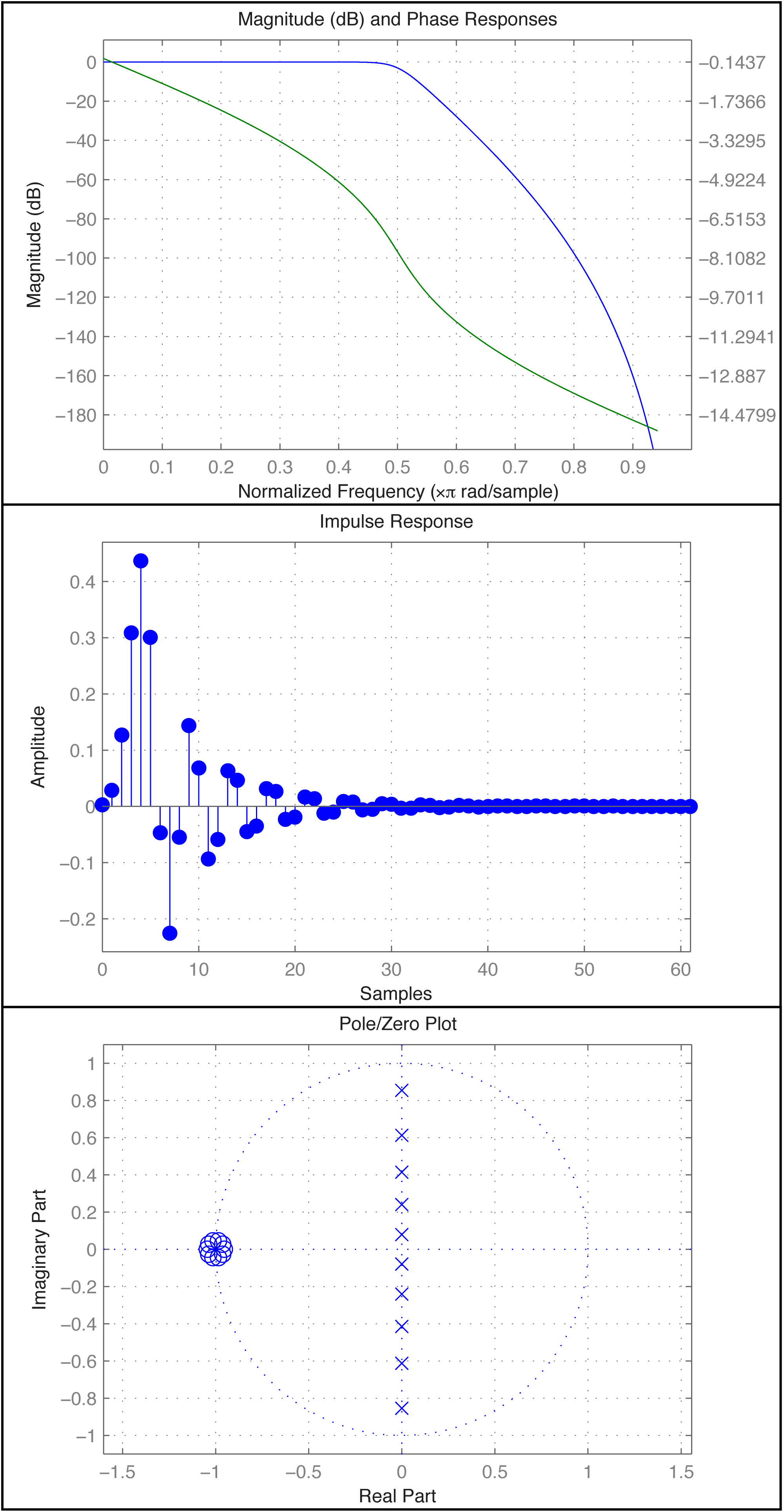
The fvtool provides a GUI through which you can see multiple views of the filter, including those in Figure 7.44. In the first figure, the blue line is the magnitude frequency response and the green line is phase.

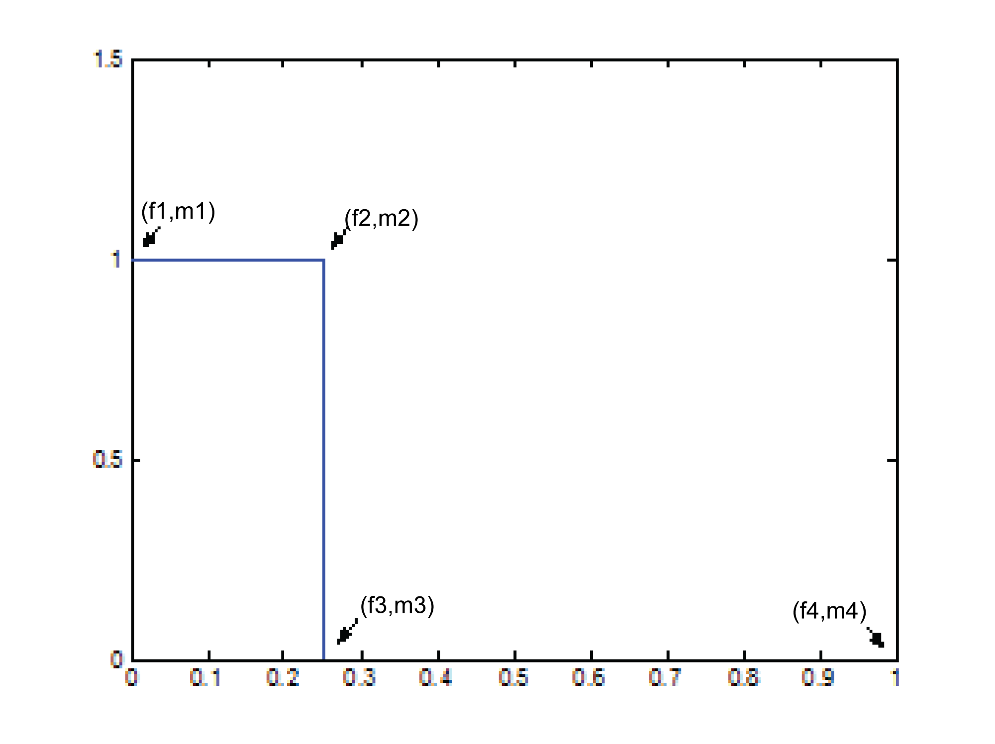
Another way to create and apply an IIR filter in MATLAB is by means of the function yulewalk. Let’s try a low-pass filter as a simple example. Figure 7.45 shows the idealized frequency response of a low-pass filter. The x-axis represents normalized frequencies, and f_c is the cutoff frequency. This particular filter allows frequencies that are up to ¼ the sampling rate to pass through, but filters out all the rest.

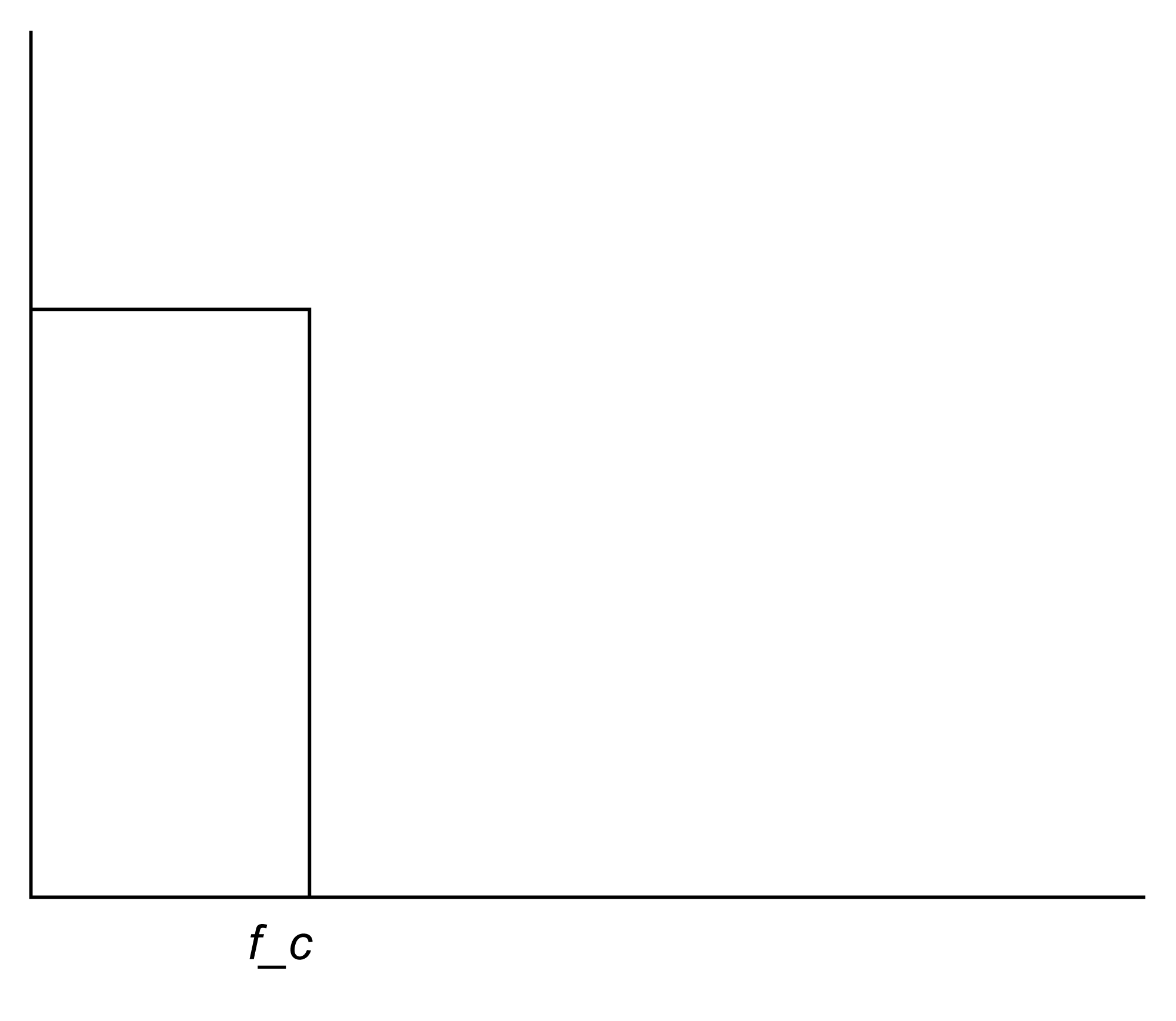
The first step in creating this filter is to store its “shape.” This information is stored in a pair of parallel vectors, which we’ll call f and m. For the four points on the graph in Figure 7.46, f stores the frequencies, and m stores the corresponding magnitudes. That is, $$\mathbf{f}=\left [ f1\; f2\; f3\; f4 \right ]$$ and $$\mathbf{m}=\left [ m1\; m2\; m3\; m4 \right ]$$, as illustrated in the figure. For the example filter we have

f = [0 0.25 0.25 1];

m = [1 1 0 0];

 

[aside]The yulewalk function in MATLAB is named for the Yule-Walker equations, a set of linear equations used in auto-regression modeling.[/aside]

Now that you have an ideal response, you use the yulewalk function in MATLAB to determine what coefficients to use to approximate the ideal response.

[a,b] = yulewalk(N,f,m)

 

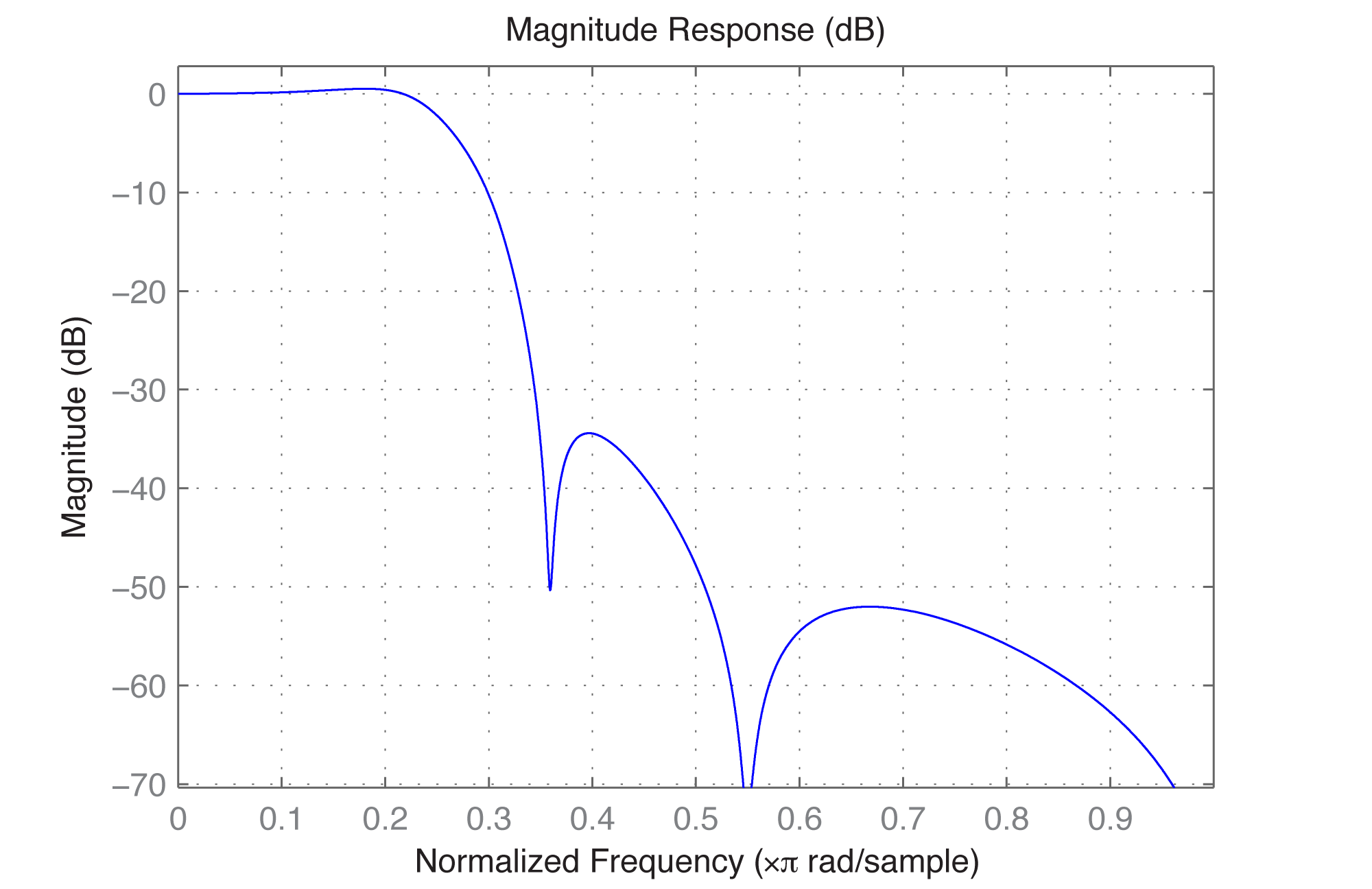
Again, an order N=6 filter is sufficient for the low-pass filter. You can use the same filter function as above to apply the filter. The resulting filter is given in Figure 7.47. Clearly, the filter cannot be perfectly created, as you can see from the large ripple after the cutoff point.

The finite counterpart to the yulewalk function is the fir2 function. Like butter, fir2 takes as input the order of the filter and two vectors corresponding to the shape of the filter’s frequency response. Thus, we can use the same f and m as before. fir2 returns the vector h constituting the filter.

h = fir2(N,f,m);

 

We need to use a higher order filter because this is an FIR. N=30 is probably high enough.

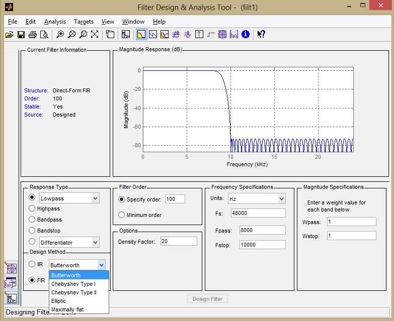
MATLAB’s extensive signal processing toolkit includes a Filter Designer with an easy-to-use graphical user interface that allows you to design the types of filters discussed in this chapter. A Butterworth filter is shown in Figure 7.48. You can adjust the parameters in the tool and see how the roll-off and ripples change accordingly. Experimenting with this tool helps you know what to expect from filters designed by different algorithms.

 

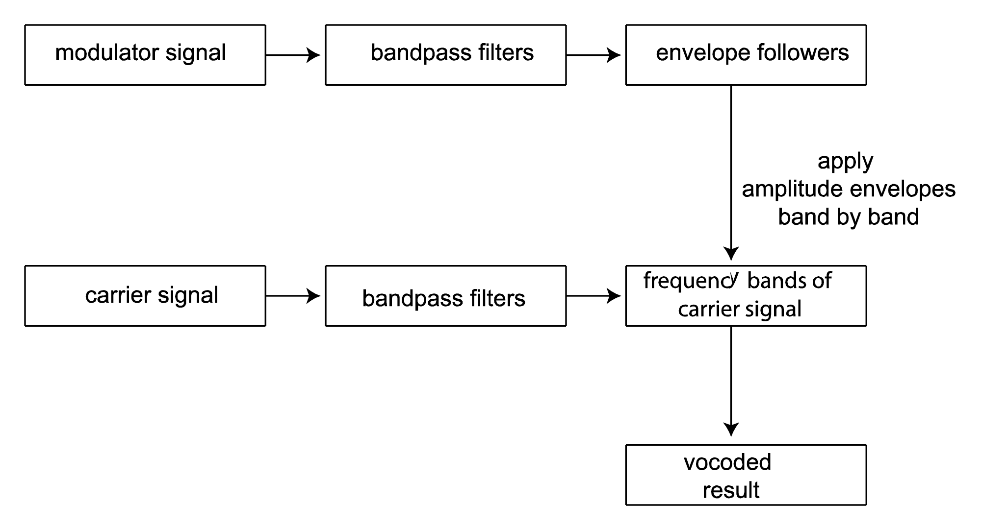
Vocoders were introduced in Section 7.1.8. The implementation of a vocoder is sketched in Algorithm 7.6 and diagrammed in Figure 7.49. The MATLAB and C++ exercises associated with this section encourage you to try your hand at the implementation.

[equation class=”algorithm” caption=”Algorithm 7.6 Sketch of an implementation of a vocoder”]

algorithm vocoder

/*

Input:

c, an array of audio samples constituting the carrier signal

m, n array of audio samples constituting the modulator signal

Output:

v, the carrier wave modulated with the modulator wave */

{

Initialize v with 0s

Divide the carrier into octave-separated frequency bands with bandpass filters

Divide the modulator into the same octave-separated frequency bands with bandpass filters for each band

use the modulator as an amplitude envelope for the carrier

}

[/equation]

[wpfilebase tag=file id=169 tpl=supplement /]

[wpfilebase tag=file id=103 tpl=supplement /]

[wpfilebase tag=file id=71 tpl=supplement /]

[wpfilebase tag=file id=101 tpl=supplement /]

Another interesting programming exercise is implementation of a pitch glide. A Risset pitch glide is an audio illusion that sounds like a constantly rising pitch. It is the aural equivalent of the visual image of a stripe on a barber pole that seems to be rising constantly. Implementing the pitch glide is suggested as an exercise for this section.

To this point, we’ve primarily considered off-line processing of audio data in the programs that we’ve asked you to write in the exercises.  This makes the concepts easier to grasp, but hides the very important issue of real-time processing, where operations have to keep pace with the rate at which sound is played.

Chapter 2 introduces the idea of audio streams.  In Chapter 2, we give a simple program that evaluates a sine function at the frequency of desire notes and writes the output directly to the audio device so that notes are played when the program runs.  Chapter 5 gives a program that reads a raw audio file and writes that to the audio device to play it as the program runs.  The program from Chapter 5 with a few modifications is given here for review.

/*Use option -lasound on compile line.  Send in number of samples and raw sound file name.*/

#include </usr/include/alsa/asoundlib.h>
#include <math.h>
#include <iostream>
using namespace std;

static char *device = "default";	/*default playback device */
snd_output_t *output = NULL;
#define PI 3.14159

int main(int argc, char *argv[])
{
        int err, numRead;
        snd_pcm_t *handle;
        snd_pcm_sframes_t frames;
        int numSamples = atoi(argv[1]);

        char* buffer = (char*) malloc((size_t) numSamples);
        FILE *inFile = fopen(argv[2], "rb");
        numRead = fread(buffer, 1, numSamples, inFile);
        fclose(inFile);   

        if ((err = snd_pcm_open(&handle, device, SND_PCM_STREAM_PLAYBACK, 0)) < 0){
            printf("Playback open error: %s\n", snd_strerror(err));
            exit(EXIT_FAILURE);
        }
        if ((err = snd_pcm_set_params(handle,
				SND_PCM_FORMAT_U8,
				SND_PCM_ACCESS_RW_INTERLEAVED,
				1,
				44100, 1, 400000) ) < 0 ){
            printf("Playback open error: %s\n", snd_strerror(err));
            exit(EXIT_FAILURE);
        }

        frames = snd_pcm_writei(handle, buffer, numSamples);
        if (frames < 0)
          frames = snd_pcm_recover(handle, frames, 0);
        if (frames < 0) {
          printf("snd_pcm_writei failed: %s\n", snd_strerror(err));
        }  
}

Program 7.1 Reading and writing raw audio data

This program uses the library function send_pcm_writei to send samples to the audio device to be played. The audio samples are read from in input file into a buffer and transmitted to the audio device without modification The variable buffer indicates where the samples are stored, and sizeof(buffer)/8 gives the number of samples given that this is 8-bit audio.

Consider what happens when you have a much larger stream of audio coming in and you want to process it in real time before writing it to the audio device. This entails continuously filling up and emptying the buffer at a rate that keeps up with the sampling rate.

Let’s do some analysis to determine how much time is available for processing based on a given buffer size. For a buffer size of N and a sampling rate of r, then $$N/r$$ seconds can be passed before additional audio data will be required for playing. For and $$N=4096$$ and $$r=44100$$, this would be $$\frac{4096}{44100}=0.0929\: ms$$. (This scheme implies that there will be latency between the input and output, at most $$N/r$$ seconds.)

What is you wanted to filter the input audio before sending it to the output? We’ve seen that filtering is more efficient in the frequency domain using the FFT. Assuming the input is in the time domain, our program has to do the following:

• convert data to the frequency domain with inverse FFT
• multiply the filter and the audio data
• convert data back to the time domain with inverse FFT
• write the data to the audio device

The computational complexity of the FFT and IFFT is $$0\left ( N\log N \right )$$, on the order of $$4096\ast 12=49152$$ operations (times 2). Multiplying the filter and the audio data is $$0\left ( N \right )$$, and writing the data to the audio devices is also $$0\left ( N \right )$$, adding on the order of the order of 2*4096 operations. This yields on the order of 106496 operations to be done in $$0.0929\; ms$$, or about $$0.9\; \mu s$$ per operation. Considering that today’s computers can do more than 100,000 MIPS (millions of instructions per second), this is not unreasonable.

We refer the reader to Boulanger and Lazzarini’s Audio Programming Book for more examples of real-time audio processing.