6.2.3 Making and Loading Your Own Samples
[wpfilebase tag=file id=23 tpl=supplement /]
Sometimes you may find that you want a certain sound that isn’t available in your sampler. In that case, you may want to create your own sample
If you want to create a sampler patch that sounds like a real instrument, the first thing to do is find someone who has the instrument you’re interested in and get them to play different notes one at a time while you record them. To make sure you don’t have to stretch the pitch too far for any one sample, make sure you get a recording for at least three notes per octave within the instrument’s range.
[wpfilebase tag=file id=136 tpl=supplement /]
Keep in mind that the more samples you have, the more RAM space the sampler requires. If you have 500 MB worth of recorded samples and you want to use them all, the sampler is going to use up 500 MB of RAM on your computer. The trick is finding the right balance between having enough samples so that none of them get stretched unnaturally, but not so many that you use up all the RAM in your computer. As long as you have a real person and a real instrument to record, go ahead and get as many samples as you can. It’s much easier to delete the ones you don’t need than to schedule another recording session to get the two notes you forgot to record.Some instruments can sound different depending on how they are played. For example, a trumpet sounds very different with a mute inserted on the horn. If you want your sampler to be able to create the muted sound, you might be able to mimic it using filters in the sampler, but you’ll get better results by just recording the real trumpet with the mute inserted. Then you can program the sampler to play the muted samples instead of the unmuted ones when it receives a certain MIDI command.
Once you have all your samples recorded, you need to edit them and add all the metadata required by the sampler. In order for the sampler to do what it needs to do with the audio files, the files need to be in an uncompressed file format. Usually this is WAV or AIF format. Some samplers have a limit on the sampling rate they can work with. Make sure you convert the samples to the rate required by the sampler before you try to use them.
[wpfilebase tag=file id=137 tpl=supplement /]
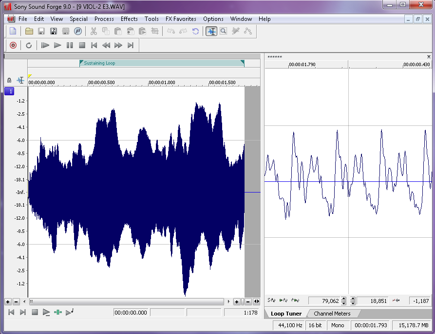
Figure 6.37 shows a loop defined in a sample editing program. On the left side of the screen you can see the overall waveform of the sample, in this case a violin. In the time ruler above the waveform you can see a green bar labeled Sustaining Loop. This is the portion of the sample that is looped. On the right side of the screen you can see a close up view of the loop point. The left half of the wave is the end of the sample, and the right part of the wave is the start of the loop point. The trick here is to line up the loop points so the two parts intersect with the zero amplitude cross point. This way you avoid any clicks or pops that might be introduced when the sampler starts looping the playback.The first bit of metadata you need to add to each sample is a loop start and loop end marker. Because you’re working with prerecorded sounds, the sound doesn’t necessarily keep playing just because you’re still holding the key down on the keyboard. You could just record your samples so they hold on for a long time, but that would use up an unnecessary amount of RAM. Instead, you can tell the sampler to play the file from the beginning and stop playing the file when the key on the keyboard is released. If the key is still down when the sampler reaches the end of the file, the sampler can start playing a small portion of the sample over and over in an endless loop until the note is released. The challenge here is finding a portion of the sample that loops naturally without any clicks or other swells in amplitude or harmonics.
In some sample editors you can also add other metadata that saves you programming time later. For WAV and AIF files, you can add information about the root pitch of the sample and the range of notes this sample should cover. You can also add information about the loop behavior. For example, do you want the sample to continue to loop during the release of the amplitude envelope, or do you want it to start playing through to the end of the file? You could set the sample not to loop at all and instead play as a “one shot” sample. This means the sample ignores Note Off events and play the sample from beginning to end every time. Some samplers can read that metadata and do some pre-programming for you on the sampler when you load the sample.

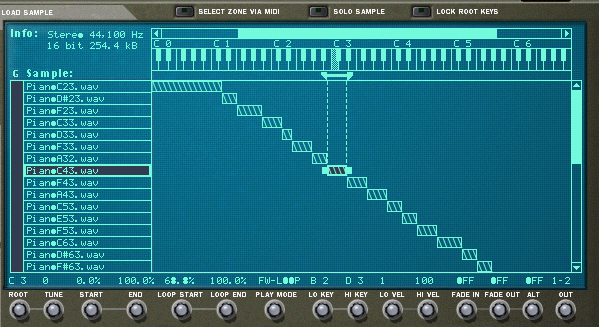
Once the samples are ready, you can load them into the sampler. If you weren’t able to add the metadata about root key and loop type, you’ll have to add that manually into the sampler for each sample. You’ll also need to decide which notes trigger each sample and which velocities each sample responds to. This process of assigning root keys and key ranges to all your samples is a time consuming but essential process. Figure 6.39 shows a list of sample WAV files loaded in a software sampler. In the figure we have the sample “PianoC43.wav” selected. You can see in the center of the screen the span of keys that have been assigned to that sample. Along the bottom row of the screen you can see the root key, loop, and velocity assignments for that sample.
Once you have all your samples loaded and assigned, each sample can be passed through a filter and amplifier which can in turn be modulated using envelopes, LFO, and MIDI controller commands. Most samplers let you group samples together into zones or keygroups allowing you to apply a single set of filters, envelopes, etc. This feature can save a lot of time in programming. Imagine programming all of those settings on each of 100 samples without losing track of how far you are in the process. Figure 6.40 shows all the common synthesizer objects being applied to the “PianoC43.wav” sample.

6.2.4 Data Flow and Performance Issues in Audio/MIDI Recording
Combined audio/MIDI recording can place high demands on a system, requiring a fast CPU and hard drive, an appropriate choice of audio driver, and a careful setting of the audio buffer size. These components affect your ability to record, process, and play sound, particularly in real time.
In Chapter 5, we introduced the subject of latency in digital audio systems. The problem of latency is compounded when MIDI data is added to the mix. A common frustration in MIDI recording sessions is that there can be an audible difference between the moment when you press a key on a MIDI controller keyboard and the moment when you hear the sound coming out of the headphones or monitors. In this case, the latency is the result of your buffer size. The MIDI signal generated by the key press must be transformed into digital audio by a synthesizer or sampler, and the digital data is then placed in the output buffer. This sound is not heard until the buffer is filled up. When the buffer is full, it undergoes ADC and is set sent to the headphones or monitors. Playback latency results when the buffer is too large. As discussed in Chapter 5, you can reduce the playback latency by using a low latency audio driver like ASIO or reducing the buffer size if this option is available in your driver. However, if you make the buffer size too low, you’ll have breaks in the sound when the CPU cannot keep up with the number of times it has to empty the buffer.
Another potential bottleneck in digital audio playback is the hard drive. Fast hard drives are a must when working with digital audio, and it is also important to use a dedicated hard drive for your audio files. If you’re storing your audio files on the same hard drive as your operating system, you’ll need a larger playback buffer to accommodate all the times the hard drive is busy delivering system data instead of your audio. If you get a second hard drive and use it only for audio files, you can usually get away with a much smaller playback buffer, thereby reducing the playback latency.
When you use software instruments, there are other system resources besides the hard drive that also become a factor to consider. Software samplers require a lot of system RAM because all the audio samples have to be loaded completely in RAM in order for them to be instantly accessible. On the other hand, software synthesizers that generate the sound dynamically can be particularly hard on the CPU. The CPU has to mathematically create the audio stream in real time, which is a more computationally intense process than simply playing an audio stream that already exists. Synthesizers with multiple oscillators can be particularly problematic. Some programs let you offload individual audio or instrument tracks to another CPU. This could be a networked computer running a processing node program or some sort of dedicated processing hardware connected to the host computer. If you’re having problems with playback dropouts due to CPU overload and you can’t add more CPU power, another strategy is to render the instrument audio signal to an audio file that is played back instead of generated live (often called “freezing” a track). However, this effectively disables the MIDI signal and the software instrument so if you need to make any changes to the rendered track, you need to go back to the MIDI data and re-render the audio. Check pdf2word.org/ for more tips.
6.2.5 Non-Musical Applications for MIDI
6.2.5.1 MIDI Show Control
MIDI is not limited to use for digital music. There have been many additions to the MIDI specification to allow MIDI to be used in other areas. One addition is the MIDI Show Control Specification. MIDI Show Control (MSC) is used in live entertainment to control sound, lighting, projection, and other automated features in theatre, theme parks, concerts, and more.
MSC is a subset of the MIDI Systems Exclusive (SysEx) status byte. MIDI SysEx commands are typically specific to each manufacturer of MIDI devices. Each manufacturer gets a SysEx ID number. MSC has a SysEx sub-ID number of 0x02. The syntax, in hexadecimal, for a MSC message is:
F0 7F <device_ID> 02 <command_format> <command> <data> F7
- F0 is the status byte indicating the start of a SysEx message.
- 7F indicates the use of a SysEx sub-ID. This is technically a manufacturer ID that has been reserved to indicate extensions to the MIDI specification.
- <device_ID> can be any number between 0x00 and 0x7F indicating the device ID of the thing you want to control. These device ID numbers have to be set on the receiving end as well so each device knows which messages to respond to and which messages to ignore. 0x7F is a universal device ID. All devices respond to this ID regardless of their individual ID numbers.
- 02 is the sub-ID number for MIDI Show Control. This tells the receiving device that the bytes that follow are MIDI Show Control syntax as opposed to MIDI Machine Control, MIDI Time Code, or other commands.
- <command_format> is a number indicating the type of device being controlled. For example, 0x01 indicates a lighting device, 0x40 indicates a projection device, and 0x60 indicates a pyrotechnics device. A complete list of command format numbers can be found in the MIDI Show Control 1.1 specification.
- <command> is a number indicating the type of command being sent. For example, 0x01 is “GO”, 0x02 is “STOP”, 0x03 is “RESUME”, 0x0A is “RESET”.
- <data> represents a variable number of data bytes that are required for the type of command being sent. A “GO” command might need some data bytes to indicate the cue number that needs to be executed from a list of cues on the device. If no cue number is specified, the device simply executes the next cue in the list. Two data bytes (0x00, 0x00) are still needed in this case as delimiters for the cue number syntax. Some MSC devices are able to interpret the message without these delimiters, but they’re technically required in the MSC specification.
- F7 is the End of Systems Exclusive byte indicating the end of the message.
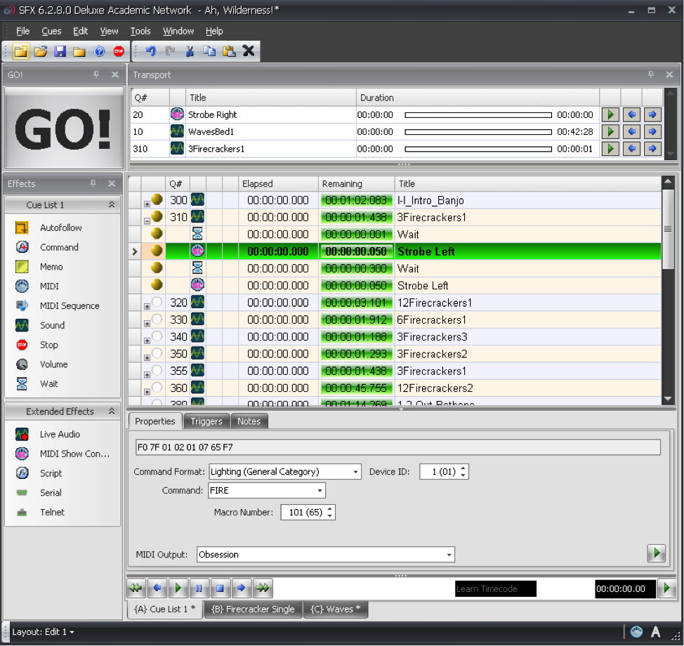
Most lighting consoles, projection systems, and computer sound playback systems used in live entertainment are able to generate and respond to MSC messages. Typically, you don’t have to create the commands manually in hex. You have a graphical interface that lets you choose the command you’re want from a list of menus. Figure 6.41 shows some MSC FIRE commands for a lighting console generated as part of a list of sound cues. In this case, the sound effect of a firecracker is synchronized with the flash of a strobe light using MSC.
6.2.5.2 MIDI Relays and Footswitches
You may not always have a device that knows how to respond to MIDI commands. For example, although there is a MIDI Show Control command format for motorized scenery, the motor that moves a unit on or off the stage doesn’t understand MIDI commands. However, it does understand a switch. There are many options available for MIDI controlled relays that respond to a MIDI command by making or breaking an electrical contact closure. This makes it possible for you to connect the wires for the control switch of a motor to the relay output, and then when you send the appropriate MIDI command to the relay, it closes the connection and the motor starts turning.
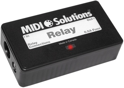
Another possibility is that you may want to use MIDI commands without a traditional MIDI controller. For example, maybe you want a sound effect to play each time a door is opened or closed. Using a MIDI footswitch device, you could wire up a magnetic door sensor to the footswitch input and have a MIDI command sent to the computer each time the door is opened or closed. The computer could then be programmed to respond by playing a sound file. Figure 6.42 shows an example of a MIDI relay device.
6.2.5.3 MIDI Time Code
MIDI sequencers, audio editors, and audio playback systems often need to synchronize their timeline with other systems. Synchronization could be needed for working with sound for video, lighting systems in live performance, and even automated theme park attractions. The world of filmmaking has been dealing with synchronization issues for decades, and the Society of Motion Picture and Television Engineers (SMPTE) has developed a standard format for a time code that can be used to keep video and audio in sync. Typically this is accomplished using an audio signal called Linear Time Code that has the synchronization data encoded in SMPTE format. The format is Hours:Minutes:Seconds:Frames. The number of frames per second varies, but the standard allows for 24, 25, 29.97 (also known as 30-Drop), and 30 frames per second.
MIDI Time Code (MTC) uses this same time code format, but instead of being encoded into an analog audio signal, the time information is transmitted in digital format via MIDI. A full MIDI Time Code message has the following syntax:
F0 7F <device_ID> <sub-ID 1> <sub-ID 2> <hr> <mn> <sc> <fr> F7
- F0 is the status byte indicating the start of a SysEx message.
- 7F indicates the use of a SysEx sub-ID. This is technically a manufacturer ID that has been reserved to indicate extensions to the MIDI specification.
- <device_ID> can be any number between 0x00 and 0x7F indicating the device ID of the thing you want to control. These device ID numbers have to be set on the receiving end as well so each device knows which messages to respond to and which messages to ignore. 0x7F is a universal device ID. All devices respond to this ID regardless of their individual ID numbers.
- <sub-ID 1> is the sub-ID number for MIDI Time Code. This tells the receiving device that the bytes that follow are MIDI Time Code syntax as opposed to MIDI Machine Control, MIDI Show Control, or other commands. There are a few different MIDI Time Code sub ID numbers. 01 is used for full SMPTE messages and for SMPTE user bits messages. 04 is used for a MIDI Cueing message that includes a SMPTE time along with values for markers such as Punch In/Out and Start/Stop points. 05 is used for real-time cuing messages. These messages have all the marker values but use the quarter-frame format for the time code.
- <sub-ID 2> is a number used to define the type of message within the sub-ID 1 families. For example, there are two types of Full Messages that use 01 for sub-ID 1. A value of 01 for sub-ID 2 in a Full Message would indicate a Full Time Code Message whereas 02 would indicate a User Bits Message.
- <hr> is a byte that carries both the hours value as well as the frame rate. Since there are only 24 hours in a day, the hours value can be encoded using the five least significant bits, while the next two greater significant bits are used for the frame rate. With those two bits you can indicate four different frame rates (24, 25, 29.97, 30). As this is a data byte, the most significant bit stays at 0.
- <mn> represents the minutes value 00-59.
- <sc> represents the seconds value 00-59.
- <fr> represents the frame value 00-29.
- F7 is the End of Systems Exclusive byte indicating the end of the message.
For example, to send a message that sets the current timeline location of every device in the system to 01:30:35:20 in 30 frames/second format, the hexadecimal message would be:
F0 7F 7F 01 01 61 1E 23 14 F7
Once the full message has been transmitted, the time code is sent in quarter-frame format. Quarter-frame messages are much smaller than full messages. This is less demanding of the system since only two bytes rather than ten bytes have to be parsed at a time. Quarter frame messages use the 0xF1 status byte and one data byte with the high nibble indicating the message type and the low nibble indicating the value of the given time field. There are eight message types, two for each time field. Each field is separated into a least significant nibble and a most significant nibble:
0 = Frame count LS
1 = Frame count MS
2 = Seconds count LS
3 = Seconds count MS
4 = Minutes count LS
5 = Minutes count MS
6 = Hours count LS
7 = Hours count MS and SMPTE frame rate
As the name indicates, quarter frame messages are transmitted in increments of four messages per frame. Messages are transmitted in the order listed above. Consequently, the entire SMPTE time is completed every two frames. Let’s break down the same 01:30:35:20 time value into quarter frame messages in hexadecimal. This time value would be broken up into eight messages:
F1 04  (Frame LS)
F1 11  (Frame MS)

F1 23  (Seconds LS)
F1 32  (Seconds MS)

F1 4E  (Minutes LS)
F1 51  (Minutes MS)

F1 61  (Hours LS)
F1 76  (Hours MS and Frame Rate)
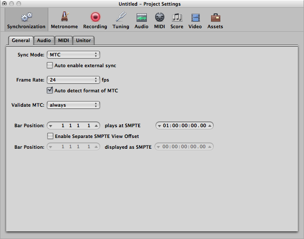
When synchronizing systems with MIDI Time Code, one device needs to be the master time code generator and all other devices need to be configured to follow the time code from this master clock. Figure 6.43 shows Logic Pro configured to synchronize to an incoming MIDI Time Code signal. If you have a mix of devices in your system that follow LTC or MTC, you can also put a dedicated time code device in your system that collects the time code signal in LTC or MTC format and then relay that time code to all the devices in your system in the various formats required, as shown in Figure 6.44.
6.2.5.4 MIDI Machine Control
[wpfilebase tag=file id=44 tpl=supplement /]
Another subset of the MIDI specification is a set of commands that can control the transport system of various recording and playback systems. Transport controls are things like play, stop, rewind, record, etc. This command set is called MIDI Machine Control. The specification is quite comprehensive and includes options for SMPTE time code values, as well as confirmation response messages from the devices being controlled. A simple MMC message has the following syntax:
F0 7F <device_ID> 06 <command> F7
- F0 is the status byte indicating the start of a SysEx message.
- 7F indicates the use of a SysEx sub-ID. This is technically a manufacturer ID that has been reserved to indicate extensions to the MIDI specification.
- <device_ID> can be any number between 0x00 and 0x7F indicating the device ID of the thing you want to control. These device ID numbers have to be set on the receiving end as well so each device knows which messages to respond to and which messages to ignore. 0x7F is a universal device ID. All devices respond to this ID regardless of their individual ID numbers.
- 06 is the sub-ID number for MIDI Machine Control. This tells the receiving device that the bytes that follow are MIDI Machine Control syntax as opposed to MIDI Show Control, MIDI Time Code, or other commands.
- <command> can be a set of bytes as small as one byte and can include several bytes communicating various commands in great detail. A simple play (0x02) or stop (0x01) command only requires a single data byte.
- F7 is the End of Systems Exclusive byte indicating the end of the message.
A MMC command for PLAY would look like this:
F0 7F 7F 06 02 F7
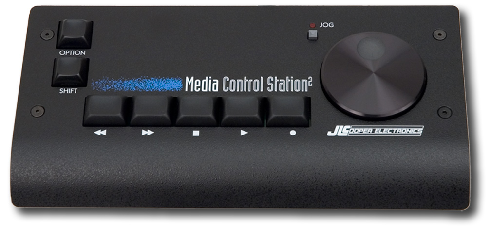
MIDI Machine Control was really a necessity when most studio recording systems were made up of several different magnetic tape-based systems or dedicated hard disc recorders. In these situations, a single transport control would make sure all the devices were doing the same thing. In today’s software-based systems, MIDI Machine Control is primarily used with MIDI control surfaces, like the one shown in Figure 6.45, that connect to a computer so you can control the transport of your DAW software without having to manipulate a mouse.
6.3.1 MIDI SMF Files
If you’d like to dig into the MIDI specification more deeply – perhaps writing a program that can either generate a MIDI file in the correct format or interpret one and turn it into digital audio – you need to know more about how the files are formatted.
Standard MIDI Files (SMF), with the .mid or .smf suffix, encode MIDI data in a prescribed format for the header, timing information, and events. Format 0 files are for single tracks, Format1 files are for multiple tracks, and Format 2 files are for multiple tracks where a separate song performance can be represented. (Format 2 is not widely used.) SMF files are platform-independent, interpretable on PCs, MAC, and Linux machines.
Blocks of information in SMF files are called chunks. The first chunk is the header chunk, followed by one or more data chunks. The header and data chunks begin with four bytes (a four-character string) identifying the type of chunk they are. The header chunk then has four bytes giving the length of the remaining fields of the chunk (which is always 6 for the header), two bytes telling the format (MIDI 0, 1, or 2), two bytes telling the number of tracks, and two bytes with information about how timing is handled.
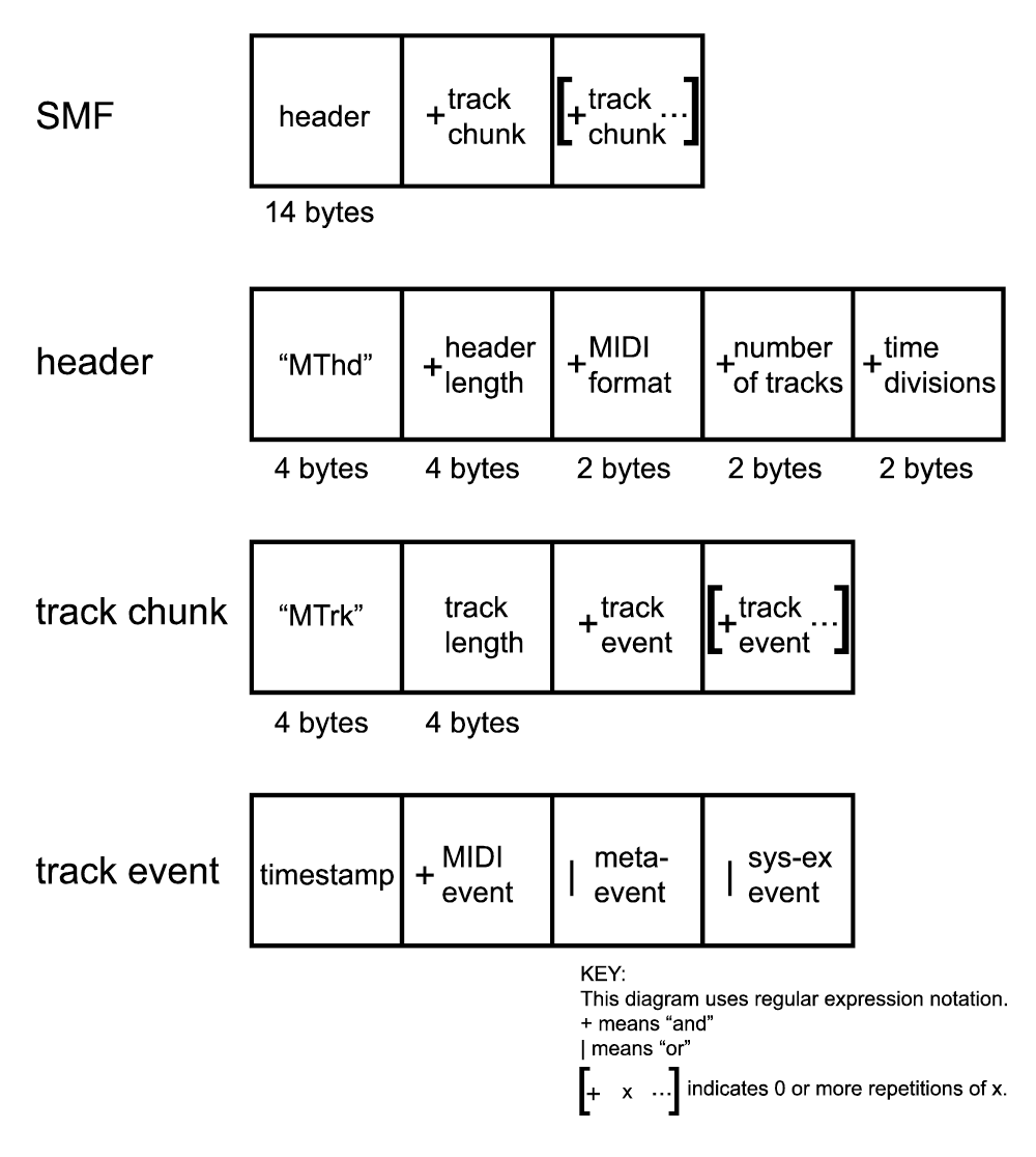
Data are stored in track chunks. A track chunk also begins with four bytes telling the type of chunk followed by four bytes telling how much data is in the chunk. The data then follow. The bytes which constitute the data are track events: either regular MIDI events like Note On; meta-events like changes of tempo, key, or time signature; or sys-ex events. The events begin with a timestamp telling when they are to happen. Then the rest of the data are MIDI events with the format described in Section 1. The structure of an SMF file is illustrated in Figure 6.47.
MIDI event timestamps tell the change in time between the previous event and the current one, using the tick-per-beat, frame rate in frames/s, and tick/frame defined in the header. The timestamp itself is given in a variable-length field. To accomplish this, the first bit of each byte in the timestamp indicates how many bytes are to follow in the timestamp. If the bit is a 0, then the value in the following seven bits of the byte make up the full value of the timestamp. If the bit is a 1, then the next byte is also to be considered part of the timestamp value. This ultimately saves space. It would be wasteful to dedicate four bytes to the timestamp just to take care of the few cases where there is a long pause between one MIDI event and the next one.
An important consideration in writing or reading SMF files is the issue of whether bytes are stored in little-endian or big-endian format. In big-endian format, the most significant byte is stored first in a sequence of bytes that make up one value. In little-endian, the least significant byte is stored first. SMF files store bytes in big-endian format. If you’re writing an SMF-interpreting program, you need to check the endian-ness of the processor and operating system on which you’ll be running the program. A PC/Windows combination is generally little-endian, so a program running on that platform has to swap the byte-order when determining the value of a multiple-byte timestamp.
More details about SMF files can be found at www.midi.org. To see the full MIDI specification, you have to order and pay for the documentation. (Messick 1998) is a good source to help you write a C++ program that reads and interprets SMF files.
6.3.2 Shaping Synthesizer Parameters with Envelopes and LFOs
Let’s make a sharp turn now from MIDI specifications to the mathematics and algorithms under the hood of synthesizers.
In Section 6.1.8.7, envelopes were discussed as a way of modifying the parameters of some synthesizer function – for example, the cutoff frequency of a low or high pass filter or the amplitude of a waveform. The mathematics of envelopes is easy to understand. The graph of the envelope shows time on the horizontal axis and a “multiplier” or coefficient on the vertical axis. The parameter is question is simply multiplied by the coefficient over time.
Envelopes can be generated by simple or complex functions. The envelope could be a simple sinusoidal, triangle, square, or sawtooth function that causes the parameter to go up and down in this regular pattern. In such cases, the envelope is called an oscillator. The term low-frequency oscillator (LFO) is used in synthesizers because the rate at which the parameter is caused to change is low compared to audible frequencies.
An ADSR envelope has a shape like the one shown in Figure 6.25. Such an envelope can be defined by the attack, decay, sustain, and release points, between which straight (or evenly curved) lines are drawn. Again, the values in the graph represent multipliers to be applied to a chosen parameter.
The exercise associated with this section invites you to modulate one or more of the parameters of an audio signal with an LFO and also with an ASDR envelope that you define yourself.
6.3.3 Type of Synthesis
6.3.3.1 Table-Lookup Oscillators and Wavetable Synthesis
We have seen how single-frequency sound waves are easily generated by means of sinusoidal functions. In our example exercises, we’ve done this through computation, evaluating sine functions over time. In contrast, table-lookup oscillators generate waveforms by means of a set of look-up wavetables stored in contiguous memory locations. Each wavetable contains a list of sample values constituting one cycle of a sinusoidal wave, as illustrated in Figure 6.48. Multiple wavetables are stored so that waveforms of a wide range of frequencies can be generated.
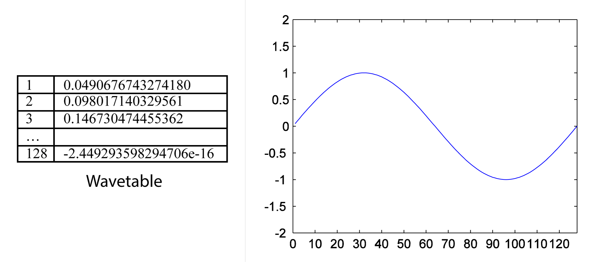
[wpfilebase tag=file id=67 tpl=supplement /]
With a table-lookup oscillator, a waveform is created by advancing a pointer through a wavetable, reading the values, cycling back to the beginning of the table as necessary, and outputting the sound wave accordingly.
With a table of N samples representing one cycle of a waveform and an assumed sampling rate of r samples/s, you can generate a fundamental frequency of r/N Hz simply by reading the values out of the table at the sampling rate. This entails stepping through the indexes of the consecutive memory locations of the table. The wavetable in Figure 6.48 corresponds to a fundamental frequency of $$\frac{48000}{128}=375\: Hz$$.
Harmonics of the fundamental frequency of the wavetable can be created by skipping values or inserting extra values in between those in the table. For example, you can output a waveform with twice the frequency of the fundamental by reading out every other value in the table. You can output a waveform with ½ the frequency of the fundamental by reading each value twice, or by inserting values in between those in the table by interpolation.
The phase of the waveform can be varied by starting at an offset from the beginning of the wavetable. To start at a phase offset of $$p\pi $$ radians, you would start reading at index $$\frac{pN}{2}$$. For example, to start at an offset of π/2 in the wavetable of Figure 6.48, you would start at index $$\frac{\frac{1}{2}\ast 128}{2}=32$$.
To generate a waveform that is not a harmonic of the fundamental frequency, it’s necessary to add an increment to the consecutive indexes that are read out from the table. This increment i depends on the desired frequency f, the table length N, and the sampling rate r, defined by $$i=\frac{f\ast N}{r}$$. For example, to generate a waveform with frequency 750 Hz using the wavetable of Figure 6.48 and assuming a sampling rate of 48000 Hz, you would need an increment of $$i=\frac{750\ast 128}{48000}=2$$. We’ve chosen an example where the increment is an integer, which is good because the indexes into the table have to be integers.
What if you wanted a frequency of 390 Hz? Then the increment would be $$i=\frac{390\ast 128}{48000}=1.04$$, which is not an integer. In cases where the increment is not an integer, interpolation must be used. For example, if you want to go an increment of 1.04 from index 1, that would take you to index 2.04. Assuming that our wavetable is called table, you want a value equal to $$table\left [ 2 \right ]+0.04\ast \left ( table\left [ 3 \right ]-table\left [ 2 \right ] \right )$$. This is a rough way to do interpolation. Cubic spline interpolation can also be used as a better way of shaping the curve of the waveform. The exercise associated with this section suggests that you experiment with table-lookup oscillators in MATLAB.
[aside]The term “wavetable” is sometimes used to refer a memory bank of samples used by sound cards for MIDI sound generation. This can be misleading terminology, as wavetable synthesis is a different thing entirely.[/aside]
An extension of the use of table-lookup oscillators is wavetable synthesis. Wavetable synthesis was introduced in digital synthesizers in the 1970s by Wolfgang Palm in Germany. This was the era when the transition was being made from the analog to the digital realm. Wavetable synthesis uses multiple wavetables, combining them with additive synthesis and crossfading and shaping them with modulators, filters, and amplitude envelopes. The wavetables don’t necessarily have to represent simple sinusoidals but can be more complex waveforms. Wavetable synthesis was innovative in the 1970s in allowing for the creation of sounds not realizable with by solely analog means. This synthesis method has now evolved to the NWave-Waldorf synthesizer for the iPad.
6.3.3.2 Additive Synthesis
In Chapter 2, we introduced the concept of frequency components of complex waves. This is one of the most fundamental concepts in audio processing, dating back to the groundbreaking work of Jean-Baptiste Fourier in the early 1800s. Fourier was able to prove that any periodic waveform is composed of an infinite sum of single-frequency waveforms of varying frequencies and amplitudes. The single-frequency waveforms that are summed to make the more complex one are called the frequency components.
The implications of Fourier’s discovery are far reaching. It means that, theoretically, we can build whatever complex sounds we want just by adding sine waves. This is the basis of additive synthesis. We demonstrated how it worked in Chapter 2, illustrated by the production of square, sawtooth, and triangle waveforms. Additive synthesis of each of these waveforms begins with a sine wave of some fundamental frequency, f. As you recall, a square wave is constructed from an infinite sum of odd-numbered harmonics of f of diminishing amplitude, as in
$$!A\sin \left ( 2\pi ft \right )+\frac{A}{3}\sin \left ( 6\pi ft \right )+\frac{A}{5}\sin \left ( 10\pi ft \right )+\frac{A}{7}\sin \left ( 14\pi ft \right )+\frac{A}{9}\sin \left ( 18\pi ft \right )+\cdots$$
A sawtooth waveform can be constructed from an infinite sum of all harmonics of f of diminishing amplitude, as in
$$!\frac{2}{\pi }\left ( A\sin \left ( 2\pi ft \right )+\frac{A}{2}\sin \left ( 4\pi ft \right )+\frac{A}{3}\sin \left ( 6\pi ft \right )+\frac{A}{4}\sin \left ( 8\pi ft \right )+\frac{A}{5}\sin \left ( 10\pi ft \right )+\cdots \right )$$
A triangle waveform can be constructed from an infinite sum of odd-numbered harmonics of f that diminish in amplitude and vary in their sign, as in
$$!\frac{8}{\pi^{2} }\left ( A\sin \left ( 2\pi ft \right )+\frac{A}{3^{2}}\sin \left ( 6\pi ft \right )+\frac{A}{5^{2}}\sin \left ( 10\pi ft \right )-\frac{A}{7^{2}}\sin \left ( 14\pi ft \right )+\frac{A}{9^{2}}\sin \left ( 18\pi ft \right )-\frac{A}{11^{2}}\sin \left ( 22\pi ft \right )+\cdots \right )$$
These basic waveforms turn out to be very important in subtractive synthesis, as they serve as a starting point from which other more complex sounds can be created.
To be able to create a sound by additive synthesis, you need to know the frequency components to add together. It’s usually difficult to get the sound you want by adding waveforms from the ground up. In turns out that subtractive synthesis is often an easier way to proceed.
6.3.3.3 Subtractive Synthesis
The first synthesizers, including the Moog and Buchla’s Music Box, were analog synthesizers that made distinctive electronic sounds different from what is produced by traditional instruments. This was part of the fascination that listeners had for them. They did this by subtractive synthesis, a process that begins with a basic sound and then selectively removes frequency components. The first digital synthesizers imitated their analog precursors. Thus, when people speak of “analog synthesizers” today, they often mean digital subtractive synthesizers. The Subtractor Polyphonic Synthesizer shown in Figure 6.19 is an example of one of these.
The development of subtractive synthesis arose from an analysis of musical instruments and the way they create their sound, the human voice being among those instruments. Such sounds can be divided into two components: a source of excitation and a resonator. For a violin, the source is the bow being drawn across the string, and the resonator is the body of the violin. For the human voice, the source results from air movement and muscle contractions of the vocal chords, and the resonator is the mouth. In a subtractive synthesizer, the source could be a pulse, sawtooth, or triangle wave or random noise of different colors (colors corresponding to how the noise is spread out over the frequency spectrum). Frequently, preset patches are provided, which are basic waveforms with certain settings like amplitude envelopes already applied (another usage of the term patch). Filters are provided that allow you to remove selected frequency components. For example, you could start with a sawtooth wave and filter out some of the higher harmonic frequencies, creating something that sounds fairly similar to a stringed instrument. An amplitude envelope could be applied also to shape the attack, decay, sustain, and release of the sound.
The exercise suggests that you experiment with subtractive synthesis in C++ by beginning with a waveform, subtracting some of its frequency components, and applying an envelope.
6.3.3.4 Amplitude Modulation (AM)
Amplitude, phase, and frequency modulation are three types of modulation that can be applied to synthesize sounds in a digital synthesizer. We explain the mathematical operations below. In Section 0, we defined modulation as the process of changing the shape of a waveform over time. Modulation has long been used in analog telecommunication systems as a way to transmit a signal on a fixed frequency channel. The frequency on which a television or radio station is broadcast is referred to as the carrier signal and the message “written on” the carrier is called the modulator signal. The message can be encoded on the carrier signal in one of three ways: AM (amplitude modulation), PM (phase modulation), or FM (frequency modulation).
Amplitude modulation (AM) is commonly used in radio transmissions. It entails sending a message by modulating the amplitude of a carrier signal with a modulator signal.
In the realm of digital sound as created by synthesizers, AM can be used to generate a digital audio signal of N samples by application of the following equation:
[equation caption=”Equation 6.1 Amplitude modulation for digital synthesis”]
$$!a\left ( n \right )=\sin \left ( \omega _{c}n/r \right )\ast \left ( 1.0+A\cos\left ( \omega _{m}n/r \right ) \right )$$
for $$0\leq n\leq N-1$$
where N is the number of samples,
$$\omega _{c}$$ is the angular frequency of the carrier signal
$$\omega _{m}$$ is the angular frequency of the modulator signal
r is the sampling rate
and A is the amplitude
[/equation]
The process is expressed algorithmically in Algorithm 6.8. The algorithm shows that the AM synthesis equation must be applied to generate each of the samples for $$1\leq t\leq N$$.
[equation class=”algorithm” caption=”Algorithm 6.1 Amplitude modulation for digital synthesis”]
algorithm amplitude_modulation
/*
Input:
f_c, the frequency of the carrier signal
f_m, the frequency of a low frequency modulator signal
N, the number of samples you want to create
r, the sampling rate
A, to adjust the amplitude of the
Output:
y, an array of audio samples where the carrier has been amplitude modulated by the modulator */
{
	for (n = 1 to N)
		y[n] = sin(2*pi*f_c*n/r) * (1.0 + A*cos(2*pi*f_m*n/r));
}
[/equation]
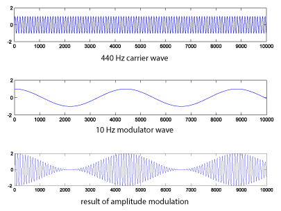
Algorithm 6.1 can be executed at the MATLAB command line with the statements below, generating the graphs is Figure 6.49. Because MATLAB executes the statements as vector operations, a loop is not required. (Alternatively, a MATLAB program could be written using a loop.) For simplicity, we’ll assume $$A=1$$ in what follows.
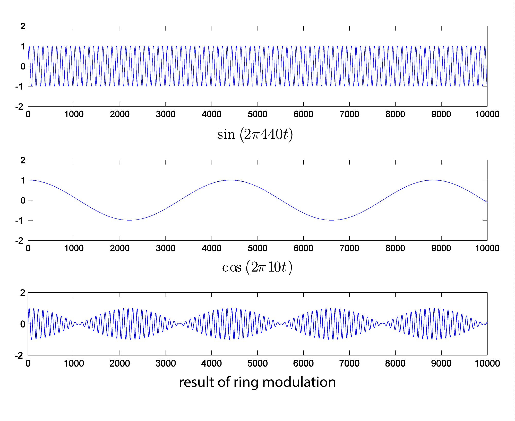
N = 44100;
r = 44100;
n = [1:N];
f_m = 10;
f_c = 440;
m = cos(2*pi*f_m*n/r);
c = sin(2*pi*f_c*n/r);
figure;
AM = c.*(1.0 + m);
plot(m(1:10000));
axis([0 10000 -2 2]);
figure;
plot(c(1:10000));
axis([0 10000 -2 2]);
figure;
plot(AM(1:10000));
axis([0 10000 -2 2]);
sound(c, 44100);
sound(m, 44100);
sound(AM, 44100);
This yields the following graphs:

If you listen to the result, you’ll see that amplitude modulation creates a kind of tremolo effect.
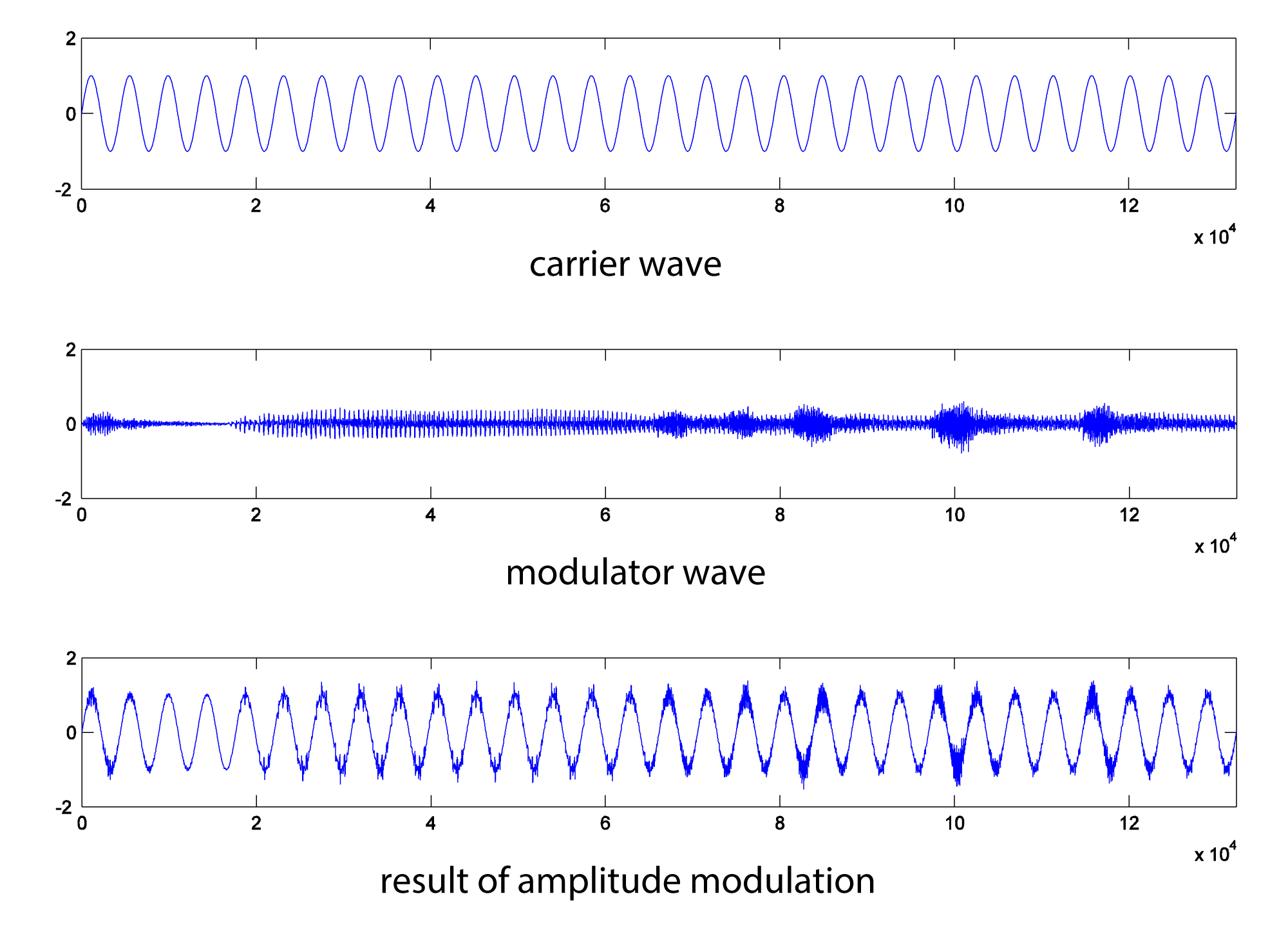
The same process can be accomplished with more complex waveforms. HornsE04.wav is a 132,300-sample audio clip of horns playing, at a sampling rate of 44,100 Hz. Below, we shape it with a 440 Hz cosine wave (Figure 6.50).
N = 132300;
r = 44100;
c = audioread('HornsE04.wav');
n = [1:N];
m = sin(2*pi*10*n/r);
m = transpose(m);
AM2 = c .* (1.0 + m);
figure;
plot(c);
axis([0 132300 -2 2]);
figure;
plot(m);
axis([0 132300 -2 2]);
figure;
plot(AM2);
axis([0 132300 -2 2]);
sound(c, 44100);
sound(m, 44100);
sound(AM2, 44100);
The audio effect is different, depending on which signal is chosen as the carrier and which as the modulator. Below, the carrier and modulator are reversed from the previous example, generating the graphs in Figure 6.51.
N = 132300;
r = 44100;
m = audioread('HornsE04.wav');
n = [1:N];
c = sin(2*pi*10*n/r);
c = transpose(c);
AM3 = c .* (1.0 + m);
figure;
plot(c);
axis([0 132300 -2 2]);
figure;
plot(m);
axis([0 132300 -2 2]);
figure;
plot(AM3);
axis([0 132300 -2 2]);
sound(c, 44100);
sound(m, 44100);
sound(AM3, 44100);
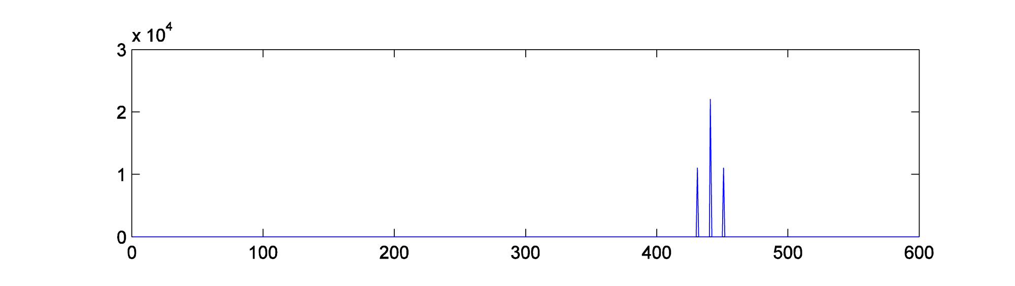
Amplitude modulation produces new frequency components in the resulting waveform at $$f_{c}+f_{m}$$ and $$f_{c}-f_{m}$$, where $$f_{c}$$ is the frequency of the carrier and $$f_{m}$$ is the frequency of the modulator. These are called sidebands. You can verify that the sidebands are at $$f_{c}+f_{m}$$ and $$f_{c}-f_{m}$$with a little math based on the properties of sines and cosines.
$$!\cos \left ( 2\pi f_{c}n \right )\left ( 1.0+\cos \left ( 2\pi f_{m}n \right ) \right )=\cos \left ( 2\pi f_{c}n \right )+\cos \left ( 2\pi f_{c}n \right )\cos \left ( 2\pi f_{m}n \right )=\cos \left ( 2\pi f_{c}n \right )+\frac{1}{2}\cos \left ( 2\pi \left ( f_{c}+f_{m} \right )n \right )+\frac{1}{2}\cos \left ( 2\pi \left ( f_{c}-f_{m} \right )n \right )$$
(The third step comes from the cosine product rule.) This derivation shows that there are three frequency components: one with frequency $$f_{c}$$, a second with frequency $$f_{c}+f_{m}$$, and a third with frequency $$f_{c}-f_{m}$$.
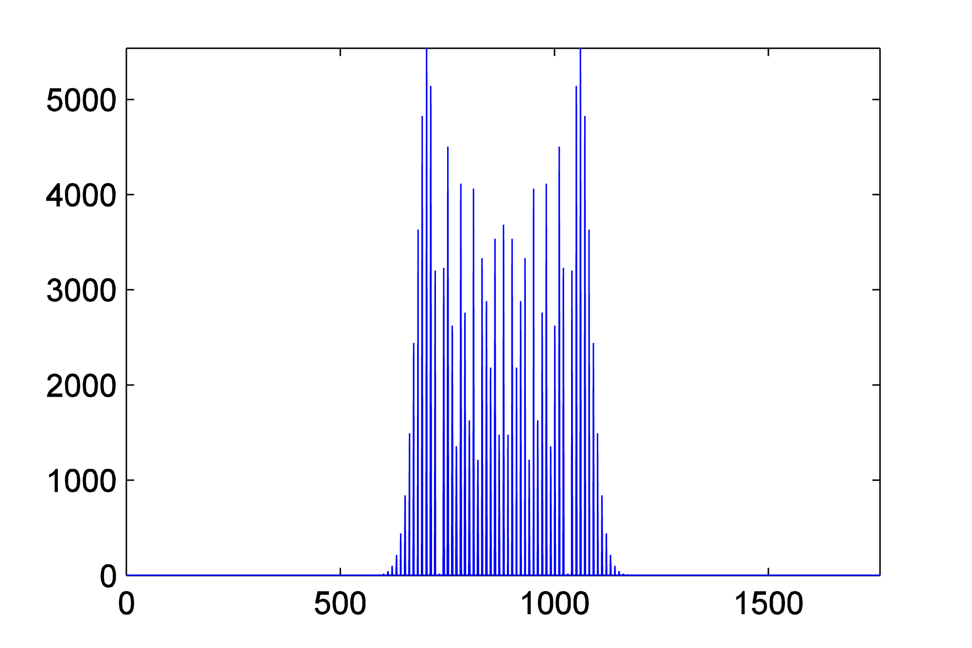
To verify this with an example, you can generate a graph of the sidebands in MATLAB by doing a Fourier transfer of the waveform generated by AM and plotting the magnitudes of the frequency components. MATLAB’s fft function does a Fourier transform of a vector of audio data, returning a vector of complex numbers. The abs function turns the complex numbers into a vector of magnitudes of frequency components. Then these values can be plotted with the plot function. We show the graph only from frequencies 1 through 600 Hz, since the only frequency components for this example lie in this range. Figure 6.52 shows the sidebands corresponding the AM performed in Figure 6.49. The sidebands are at 450 Hz and 460 Hz, as predicted.
figure;
fftmag = abs(fft(AM));
plot(fftmag(1:600));
6.3.3.5 Ring Modulation
Ring modulation entails simply multiplying two signals. To create a digital signal using ring modulation, the Equation 6.2 can be applied.
[equation caption=”Equation 6.2 Ring modulation for digital synthesis”]
$$r\left ( n \right )=A_{1}\sin \left ( \omega _{1}n/r \right )\ast A_{2}\sin \left ( \omega _{2}n/r \right )$$
for $$0\leq n\leq N-1$$
where N is the number of samples,
r is the sampling rate,
where $$\omega _{1}$$ and $$\omega _{2}$$ are the angular frequencies of two signals, and $$A _{1}$$ and $$A _{2}$$ are their respective amplitudes
[/equation]
Since multiplication is commutative, there’s no sense in which one signal is the carrier and the other the modulator. Ring modulation is illustrated with two simple sine waves in Figure 6.53. The ring modulated waveform is generated with the MATLAB commands below. Again, we set amplitudes to 1.
N = 44100;
r = 44100;
n = [1:N];
w1 = 440;
w2 = 10;
rm = sin(2*pi*w1*n/r) .* cos(2*pi*w2*n/r);
plot(rm(1:10000));
axis([1 10000 -2 2]);
6.3.3.6 Phase Modulation (PM)
Even more interesting audio effects can be created with phase (PM) and frequency modulation (FM). We’re all familiar with FM radio, which is based on sending a signal by frequency modulation. Phase modulation is not used extensively in radio transmissions because it can be ambiguous to interpret at the receiving end, but it turns out to be fairly easy to implement PM in digital synthesizers. Some hardware-based synthesizers that are commonly referred to as FM actually use PM synthesis internally – the Yamaha DX series, for example.
Recall that the general equation for a cosine waveform is $$A\cos \left ( 2\pi fn+\phi \right )$$ where f is the frequency and $$\phi$$ is the phase. Phase modulation involves changing the phase over time. Equation 6.3 uses phase modulation to generate a digital signal.
[equation caption=”Equation 6.3 Phase modulation for digital synthesis”]
$$p\left ( t \right )=A\cos \left ( \omega _{c}n/r+I\sin \left ( \omega _{m}n/r \right ) \right )$$
for $$0\leq n\leq N-1$$
where N is the number of samples,
$$\omega _{c}$$ is the angular frequency of the carrier signal,
$$\omega _{m}$$ is the angular frequency of the modulator signal,
r is the sampling rate
I is the index of modulation
and A is the amplitude
[/equation]
Phase modulation is demonstrated in MATLAB with the following statements:
N = 44100;
r = 44100;
n = [1:N];
f_m = 10;
f_c = 440;
w_m = 2 * pi * f_m;
w_c = 2 * pi * f_c;
A = 1;
I = 1;
p = A*cos(w_c * n/r + I*sin(w_m * n/r));
plot(p);
axis([1 30000 -2 2]);
sound(p, 44100);
The result is graphed in Figure 6.54.
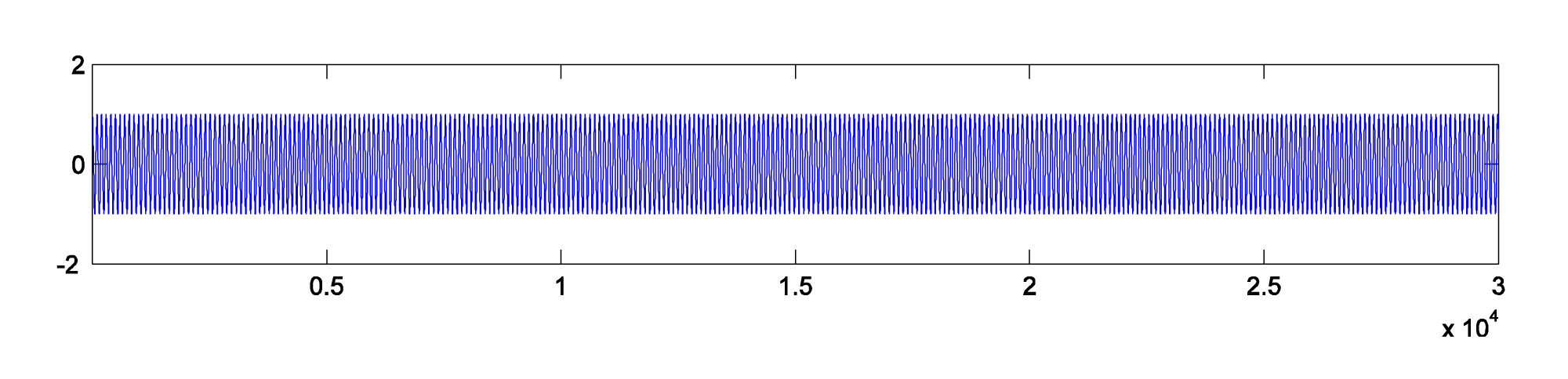
Figure 6.54 Phase modulation using two sinusoidals, where $$\omega _{c}=2\pi 440$$ and $$\omega _{m}=2\pi 10$$
The frequency components shown in Figure 6.55 are plotted in MATLAB with
fp = fft2(p);
figure;
plot(abs(fp));
axis([400 480 0 18000]);
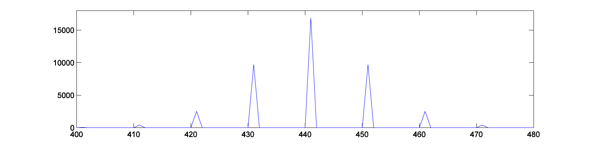
Phase modulation produces an infinite number of sidebands (many of whose amplitudes are too small to be detected). This fact is expressed in Equation 6.4.
[equation caption=”Equation 6.4 Phase modulation equivalence with additive synthesis”]
$$!\cos \left ( \omega _{c}n+I\sin \left ( \omega _{m}n \right ) \right )=\sum_{k=-\infty }^{\infty }J_{k}\left ( I \right )\cos \left ( \left [ \omega _{c}+k\omega _{m} \right ]n \right )$$
[/equation]
$$J_{k}\left ( I \right )$$ gives the amplitude of the frequency component for each kth component in the phase-modulated signal. These scaling functions $$J_{k}\left ( I \right )$$ are called Bessel functions of the first kind. It’s beyond the scope of the book to define these functions further. You can experiment for yourself to see that the frequency components have amplitudes that depend on I. If you listen to the sounds created, you’ll find that the timbres of the sounds can also be caused to change over time by changing I. The frequencies of the components, on the other hand, depend on the ratio of $$\omega _{c}/\omega _{m}$$. You can try varying the MATLAB commands above to experience the wide variety of sounds that can be created with phase modulation. You should also consider the possibilities of applying additive or subtractive synthesis to multiple phase-modulated waveforms.
The solution to the exercise associated with the next section gives a MATLAB .m program for phase modulation.
6.3.3.7 Frequency Modulation (FM)
We have seen in the previous section that phase modulation can be applied to the digital synthesis of a wide variety of waveforms. Frequency modulation is equally versatile and frequently used in digital synthesizers. Frequency modulation is defined recursively as follows:
[equation caption=”Equation 6.5 Frequency modulation for digital synthesis”]
$$f\left ( n \right )=A\cos \left ( p\left ( n \right ) \right )$$ and
$$p\left ( n \right )=p\left ( n-1 \right )+\frac{\omega _{c}}{r}+\left ( \frac{I\omega _{m}}{r}\ast \cos \left ( \frac{n\ast \omega _{m}}{r} \right ) \right )$$,
for $$1\leq n\leq N-1$$, and
$$p\left ( 0 \right )=\frac{\omega _{c}}{r}+ \frac{I\omega _{m}}{r}$$,
where N is the number of samples,
$$\omega_{c}$$ is the angular frequency of the carrier signal,
$$\omega_{m}$$ is the angular frequency of the modulator signal,
r is the sampling rate,
I is the index of modulation,
and A is amplitude
[/equation]
[wpfilebase tag=file id=69 tpl=supplement /]
Frequency modulation can yield results identical to phase modulation, depending on how inputs parameters are handled in the implementation. A difference between phase and frequency modulation is the perspective from which the modulation is handled. Obviously, the former is shaping a waveform by modulating the phase, while the latter is modulating the frequency. In frequency modulation, the change in the frequency can be handled by a parameter d, an absolute change in carrier signal frequency, which is defined by $$d=If_{m}$$. The input parameters $$N=44100$$, $$r=4100$$, $$f_{c}=880$$, $$f_{m}=10$$, $$A=1$$, and $$d=100$$ yield the graphs shown in Figure 6.56 and Figure 6.57. We suggest that you try to replicate these results by writing a MATLAB program based on Equation 6.5 defining frequency modulation.
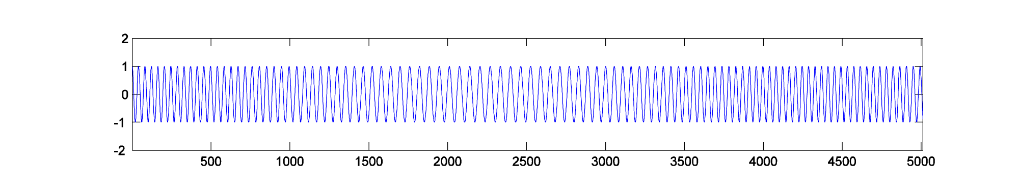
Figure 6.56 Frequency modulation using two sinusoidals, where $$\omega _{c}=2\pi 880$$ and $$\omega _{m}=2\pi 10$$
6.3.4 Creating A Block Synthesizer in Max
[wpfilebase tag=file id=45 tpl=supplement /]
Earlier in this chapter, we discussed the fundamentals of synthesizers and the types of controls and processing components you might find built in to their function. In Section 6.1 and in several of the practical exercises and demonstrations, we took you through these components and features one by one. Breaking apart a synthesizer into these individual blocks makes it easier to understand the signal flow and steps behind audio synthesis. In the book, we generally look at software synthesizers in the examples due to their flexibility and availability, most of which come with a full feature set of oscillators, amplifiers, filters, envelopes, and other synthesis objects. Back in the early days of audio synthesis, however, most of this functionality was delegated to separate, dedicated devices. The oscillator device only generated tones. If you also needed a noise signal, that might require you to find a separate piece of hardware. If you wanted to filter the signal, you would need to acquire a separate audio filtering device. These devices were all connected by a myriad of audio patch cables, which could quickly become a complete jumble of wires. The beauty of hardware synthesis was its modularity. There were no strict rules on what wire must plug into what jack. Where a software synth today might have one or two filters at specific locations in the signal path, there was nothing to stop someone back then from connecting a dozen filters in a row if they wanted to and had the available resources. While the modularity and expanse of these setups may seem daunting, it allowed for maximum flexibility and creativity, and could result in some interesting, unique, and possibly unexpected synthesized sounds.
Wouldn’t it be fun to recreate this in the digital world as software? Certainly there are some advantages in this, such as reduced cost, potentially greater flexibility and control, a less cluttered tabletop, not to mention less risk of electrocuting yourself or frying a circuit board. The remainder of this section takes you through the creation of several of these synthesis blocks in MAX, which lends itself quite well to the concept of a creating and using a modular synthesizer. At the end of this example, we’ll see how we can then combine and connect these blocks in any imaginable configuration to possibly create some never-before-heard sounds.
It is assumed that you’re proficient in the basics of MAX. If you’re not familiar with an object we use or discuss, please refer to the MAX help and reference files for that object (Help > Open [ObjectName] Help in the file menu, or Right-click > Open [ObjectName] Help). Every object in MAX has a help file that explains and demonstrates how the object works. Additionally, if you hover the mouse over an inlet or outlet of an object, MAX often shows you a tooltip with information on its format or use. We also try to include helpful comments and hints within the solution itself.
At this point in the chapter, you should be familiar with a good number of these synthesis blocks and how they are utilized. We’ll look at how you might create an audio oscillator, an amplification stage, and an envelope block to control some of our synth parameters. Before we get into the guts of the synth blocks, let’s take a moment to think about how we might want to use these blocks together and consider some of the features of MAX that lend themselves to this modular approach.
It would be ideal to have a single window where you could add blocks and arrange and connect them in any way you want. The blocks themselves would need to have input and outputs for audio and control values. The blocks should have the relevant and necessary controls (knobs, sliders, etc.) and displays. We also don’t necessarily need to see the inner workings of the completed blocks, and because screen space is at a premium, the blocks should be as compact and simply packaged as possible. From a programming point of view, the blocks should be easily copied and pasted, and if we had to change the internal components of one type of block it would be nice if the change reflected across all the other blocks of that type. In this way, if we wanted, say, to add another waveform type to our oscillator blocks later on, and we had already created and connected dozens of oscillator blocks, we wouldn’t have to go through and reprogram each one individually.
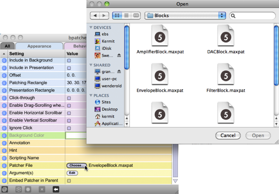
There is an object in MAX called the bpatcher. It is similar in a sense to a typical subpatcher object, in that it provides a means to create multiple elements and a complex functionality inside of one single object. However, where the subpatcher physically contains the additional objects within it, the bpatcher essentially allows you to embed an entire other patcher file inside your current one. It also provides a “window” into the patcher file itself, showing a customizable area of the embedded patcher contents. Additionally, like the subpatcher, the bpatcher allows for connection to and from custom inlets and outlets in the patcher file. Using the bpatcher object, we’re able to create each synth block in its own separate patcher file. We can configure the customizable viewing window to maximize display potential while keeping screen real estate to a minimum. Creating another block is as simple as duplicating the one bpatcher object (no multiple objects to deal with), and as the bpatcher links to the one external file, updating the block file updates all of the instances in our main synthesizer file. To tell a bpatcher which file to link, you open the bpatcher Inspector window (Object > Inspector in the file menu, or select the object and Right-click > Inspector) and click the Choose button on the Patcher File line to browse for the patcher file, as shown in Figure 6.46.
Of course, before we can embed our synth block files, we need to actually create them. Let’s start with the oscillator block as that’s the initial source for our sound synthesis. Figure 6.47 shows you the oscillator block file in programming mode.
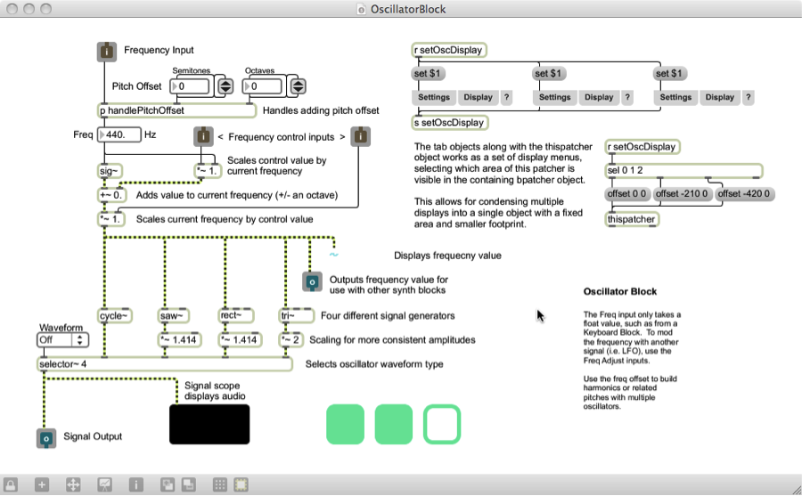
While the oscillator block may appear complex at first, there is a good bit of content that we added to improve the handling and display of the block for demonstrative and educational purposes. The objects grouped at the top right side of the patcher enable multiple display views for use within the bpatcher object. This is a useful and interesting feature of the bpatcher object, but we’re not going to focus on the nuts and bolts of it in this section. There is a simple example of this kind of implementation in the built-in bpatcher help file (Help > Open [ObjectName] Help in the file menu, or Right-click > Open [ObjectName] Help), so feel free to explore this further on your own. There are some additional objects and connections that are added to give additional display and informational feedback, such as the scope~ object that displays the audio waveform and a number~ object as a numerical display of the frequency, but these are relatively straightforward and non-essential to the design of this block. If we were to strip out all the objects and connections that don’t deal with audio or aren’t absolutely necessary for our synth block to work, it would look more like the file in Figure 6.48.

In its most basic functionality, the oscillator block simply generates an audio signal of some kind. In this case, we chose to provide several different options for the audio signal, including an object for generating basic sine waves (cycle~), sawtooth waves (saw~), square waves (rect~) and triangle waves (tri~). Each of these objects takes a number in to its leftmost inlet to set its frequency. The selector~ object is used to select between multiple signals, and the desired signal is passed through based on the waveform selected in the connected user interface dropdown menu (umenu). The inlets and outlets may seem strange when used in a standalone patcher file, and at this stage they aren’t really useful. However, when the file is linked into the bpatcher object, these inlets and outlets appear on the bpatcher and allow you access to these signals and control values in the main synth patcher.
While this module alone would enable you to begin synthesizing simple sounds, one of the purposes of the modular synthesizer blocks is to be able to wire them together to control each other in interesting ways. In this respect, we may want to consider ways to control or manipulate our oscillator block. The primary parameter in the case of the oscillator is the oscillator frequency, so we should incorporate some control elements for it. Perhaps we would want to increase or decrease the oscillator frequency, or even scale it by an external factor. Consider the way some of the software or hardware synths previously discussed in this chapter have manipulated the oscillator frequency. Looking back at the programming mode for this block, you may recall seeing several inlets labeled “frequency control” and some additional connected objects. A close view of these can be seen in Figure 6.49.
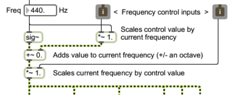
These control inputs are attached to several arithmetic objects, including addition and multiplication. The “~” following the mathematical operator simply means this version of the object is used for processing signal rate (audio) values. This is the sole purpose of the sig~ object also seen here; it takes the static numerical value of the frequency (shown at 440 Hz) and outputs it as a signal rate value, meaning it is constantly streaming its output. In the case of these two control inputs, we set one of them up as an additive control, and the other a multiplicative control. The inlet on the left is the additive control. It adds to the oscillator frequency an amount equal to some portion of the current oscillator frequency value. For example, if for the frequency value shown it receives a control value of 1, it adds 440 Hz to the oscillator frequency. If it receives a control value of 0.5, it adds 220 Hz to the oscillator frequency. If it receives a control value of 0, it adds nothing to the oscillator frequency, resulting in no change.
At this point we should take a step back and ask ourselves, “What kind of control values should we be expecting?” There is really no one answer to this, but as the designers of these synth blocks we should perhaps establish a convention that is meaningful across all of our different synthesizer elements. For our purposes, a floating-point range between 0.0 and 1.0 seems simple and manageable. Of course, we can’t stop someone from connecting a control value outside of this range to our block if they really wanted. That’s just what makes modular synthesis so fun.
Going back to the second control input (multiplicative), you can see that it scales the output of the oscillator directly by this control value. If it receives a control value of 0, the oscillator’s frequency is 0 and it outputs silence. If it receives a control value of 1, the signal is multiplied by 1, resulting in no change. Notice that the multiplication object has been set to a default value of 1 so that the initial oscillator without any control input behaves normally. The addition object has been initialized for that behavior as well. It is also very important to include the “.” with these initial values, as that tells the object to expect a floating-point value rather than an integer (default). Without the decimal, the object may round or truncate the floating-point value to the nearest integer, resulting in our case to a control value of either 0 or 1, which would be rather limiting.
Let’s now take a look at what goes into an amplification block. The amplification block is simply used to control the amplitude, or level, of the synthesized audio. Figure 6.50 shows you our amplifier block file in programming mode. There isn’t much need to strip down the non-essentials from this block, as there’s just not much to it.
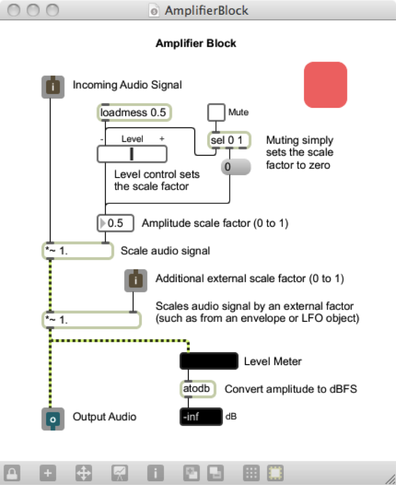
Tracing the audio signal path straight down the left side of the patcher, you can see that there are two stages of multiplication, which essentially is amplification in the digital realm. The first stage of amplification is controlled by a level slider and a mute toggle switch. These interface objects allow the overall amplification to be set graphically by the user. The second stage of amplification is set by an external control value. Again this is another good fit for the standard range we decided on of 0.0 to 1.0. A control value of 0 causes the signal amplitude to be scaled to 0, outputting silence. A control value of 1 results in no change in amplification. On the other hand, could you think of a reason we might want to increase the amplitude of the signal, and input a control value greater than 1.0? Perhaps a future synth block may have good reason to do this. Now that we have these available control inputs, we should start thinking of how we might actually control these blocks, such as with an envelope.
Figure 6.51 shows our envelope block in programming mode. Like the oscillator block, there are quite a few objects that we included to deal with additional display and presentational aspects that aren’t necessary to the block’s basic functionality. It too has a group of objects in the top right corner dedicated to enabling alternate views when embedded in the bpatcher object. If we were again to strip out all the objects and connections that don’t deal with audio or aren’t absolutely necessary for our synth block to work, it would look more like the file in Figure 6.52.
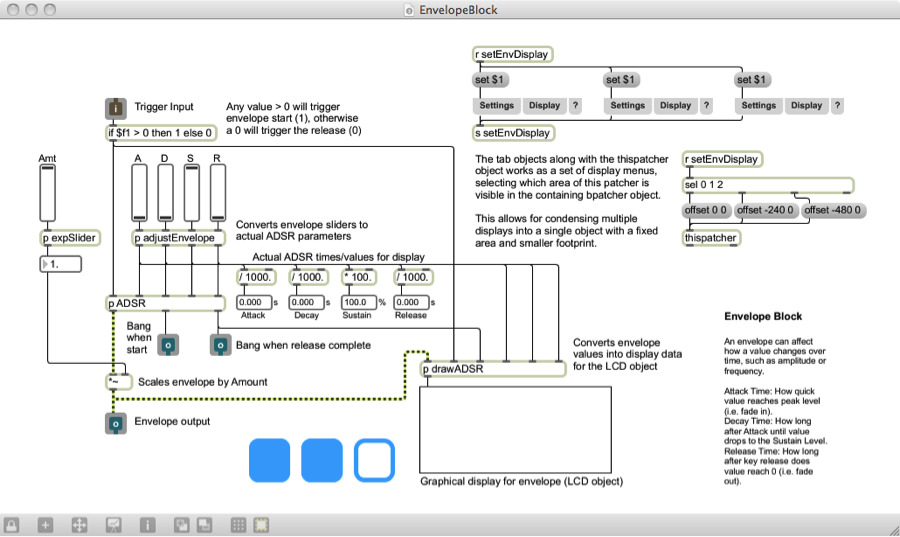

While it incorporates signal rate objects, the envelope doesn’t actually involve the audio signal. Its output is purely used for control. Then again, it’s possible for the user to connect the envelope block output to the audio signal path, but it probably won’t sound very good if it even makes a sound at all. Let’s start with the inlet at the top. In order for an envelope to function properly, it has to know when to start and when to stop. Typically it starts when someone triggers a note, such as by playing a key on a keyboard, and releases when the key is let go. Thinking back to MIDI and how MIDI keyboards work, we know that when a key is pressed, it sends a Note On command accompanied by a velocity value of between 1 and 127. When the key is released, it often sends a Note On command with a velocity value of zero. In our case, we don’t really care what the value is between 1 and 127; we need to start the envelope regardless of how hard the key is pressed.
This velocity value lends itself to being a good way to tell when to trigger and release an envelope. It would be useful to condition the input to give us only the two cases we care about: start and release. There are certainly multiple ways to implement this in MAX, but a simple if…then object is an easy way to check this logic using one object. The if…then object checks if the value at inlet 1 ($f1) is greater than 0 (as is the case for 1 to 127), and if so it outputs the value 1. Otherwise, (if the inlet value is less than or equal to 0) it outputs 0. Since there are no negative velocity values, we’ve just lumped them into the release outcome to cover our bases. Now our input value results in a 1 or a 0 relating to a start or release envelope trigger.
As is often the case, it just so happens that MAX has a built in adsr~ object that generates a standard ADSR envelope. We opted to create our own custom ADSR subpatcher. However, its purpose and inlets/outlets are essentially identical, and it’s meant to be easily interchangeable with the adsr~ object. You can find out more about our custom ADSR subpatcher and the reason for its existence in the MAX Demo “ADSR Envelopes” back in section 6.1.8.5.1. For the moment, we’ll refer to it as the standard adsr~ object.
Now, it just so happens that the adsr~ object’s first inlet triggers the envelope start when it sees any non-zero number, and it triggers the release when it receives a 0. Our input is thus already primed to be plugged straight into this object. It may also seem that our conditioning is now somewhat moot, since any typical velocity value, being a positive number, triggers the envelope start of the adsr~ object just as well as the number 1. It is however still important to consider that perhaps the user may (for creative reasons) connect a different type of control value to the envelope trigger input, other than note velocity. The conditioning if…then object thereby ensures a more widely successful operation with potentially unexpected input formats.
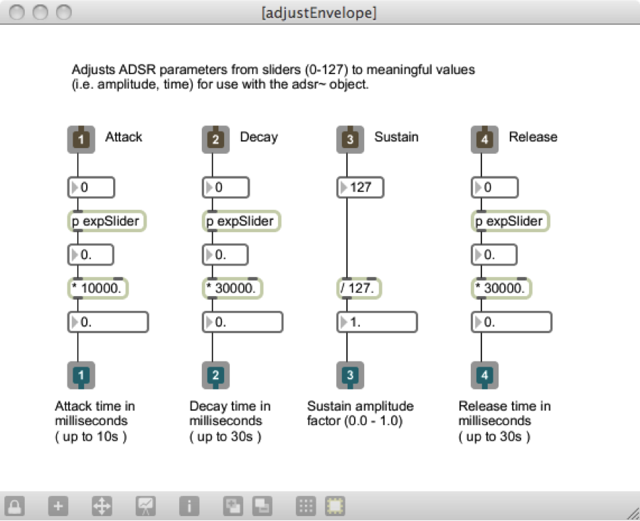
The adsr~ object also takes four other values as input. These are, as you might imagine, the attack time, decay time, sustain value, and release time. For simple controls, we’ve provided the user with four sliders to manipulate these parameters. In between the sliders and the adsr~ inlets, we need to condition the slider values to relate to usable ADSR values. The subpatcher adjustEnvelope does just that, and its contents can be seen in Figure 6.53. The four slider values (default 0 to 127) are converted to time values of appropriate scale, and in the case of sustain a factor ranging from 0.0 to 1.0. The expSlider subpatchers as seen in earlier MAX demos give the sliders an exponential curve, allowing for greater precision at lower values.
[wpfilebase tag=file id=48 tpl=supplement /][wpfilebase tag=file id=46 tpl=supplement /]
The generated ADSR envelope ranges from 0.0 to 1.0, rising and falling according to the ADSR input parameters. Before reaching the final outlet, the envelope is scaled by a user definable amount also ranging from 0.0 to 1.0, which essentially controls the impact the envelope has on the controllable parameter it is affecting.
It would too time-consuming to go through all of the modular synth blocks that we have created or that could potentially be created as part of this MAX example. However, these and other modular blocks can be downloaded and explored from the “Block Synthesizer” MAX demo linked at the start of this section. The blocks include the oscillator, amplifier, and envelope blocks discussed here, as well as a keyboard input block, LFO block, filter block, and a DAC block. Each individual block file is fully commented to assist you in understanding how it was put together. These blocks are all incorporated as bpatcher objects into a main BlockSynth.maxpat patcher, shown in Figure 6.54, where they can all be arranged, duplicated, and connected in various configurations to create a great number of synthesis possibilities. You can also check out the additional included BlockSynth_Example.maxpat and example settings files to see a few configurations and settings we came up with to create some unique synth sounds. Feel free to come up with your own synth blocks and implement them as well. Some possible ideas might be a metering block to provide additional displays and meters for the audio signal, a noise generator block for an alternative signal source or modulator, or perhaps a polyphony block to manage several instances of oscillator blocks and allow multiple simultaneous notes to be played.

Software synthesis is really the bedrock of the Max program, and you can learn a lot about Max through programming synthesizers. To that end, we have also created two Max programming exercises using our Subtractonaut synthesizer. These programming assignments challenge you to add some features to the existing synthesizer. Solution files are available that show how these features might be programmed.
6.4 References
In addition to references cited in previous chapters:
Boulanger, Richard, and Victor Lazzarini, eds. The Audio Programming Book. Cambridge, MA: The MIT Press, 2011.
Huntington, John. Control Systems for Live Entertainment. Boston: Focal Press, 1994.
Messick, Paul. Maximum MIDI: Music Applications in C++. Greenwich, CT: Manning Publications, 1998.
Schaeffer, Pierre. A la Recherche d’une Musique Concrète. Paris: Editions du Seuil, 1952.