3.3.3 Experimenting with Music in Max
Max (and its open source counterpart, PD) is a powerful environment for experimenting with sound and music. We use one of our own learning supplements, a Max patcher for generating scales (3.1.4), as an example of the kinds of programs you can write.
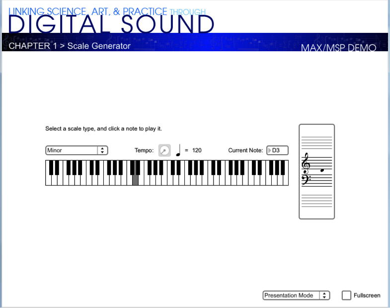
When you open this patcher, it is in presentation mode (Figure 3.47), as indicated by the drop-down menu in the bottom right corner. In presentation mode, the patcher is laid out in a user-friendly format, showing only the parts of the interface that you need in order to run the tutorial, which in this case allows you to generate major and minor scales in any key you choose. You can change to programming mode (Figure 3.48) by choosing this option from the drop-down menu.
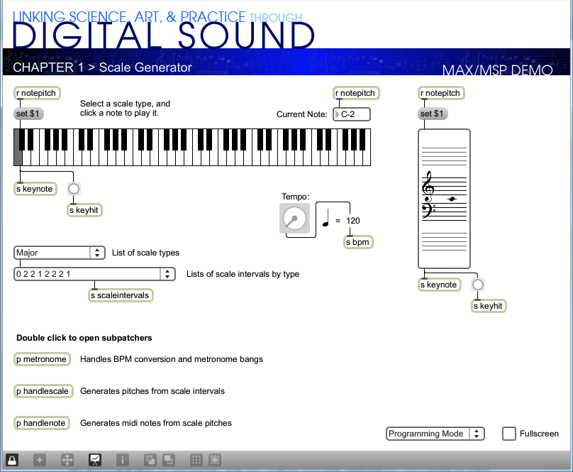
Programming mode reveals more of the Max objects used in the program. You can now see that the scale-type menu is connected to a list object. This list changes in accordance with the selection, each time giving the number of semitones between consecutive notes on the chosen type of scale. You can also see that the program is implemented with a number of send, receive, and patcher objects. Send and receive objects pass data between them, as the names imply. Objects named s followed by an argument, as in s notepitch, are the send objects. Objects named r followed by an argument, as in r notepitch, are the receive objects. Patcher objects are “subpatchers” within the main program, their details hidden so that the main patcher is more readable. You can open a patcher object in programming mode by double-clicking on it. The metronome, handlescale, and handlenote patcher objects are open in Figure 3.49, Figure 3.50, and Figure 3.51.

In this example, you still can’t see the details of how messages are being received and processed. To do so, you have to unlock the main patcher window by clicking the lock icon in the bottom left corner. This puts you in a mode where you can inspect and even edit objects. The main patcher is unlocked in Figure 3.52. You must have the full Max application, not just the runtime, to go into full programming mode.

With all the patcher objects exposed and the main patcher unlocked, you can now see how the program is initialized and how the user is able to trigger the sending and receiving of messages by selecting from a menu, turning the dial to set a tempo, and clicking the mouse on the keyboard display. Here’s how the program runs:
- The loadbang object is triggered when the program begins. It is used to initialize the tempo to 120 bpm and to set the default MIDI output device. Both of these can be changed by the user.
- The user can select a type of scale from a menu. The list of intervals is set accordingly and sent in the variable scalesintervals, to be received by the handlescale patcher object.
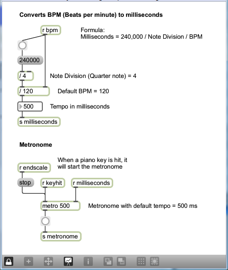
- The user can select a tempo through the dial object. The input value is sent to the metronome patcher object to determine the timing of the notes played in the scale.
- The user can click a key on the keyboard object. This initiates the playing of a scale by sending a keyhit message to both the metronome and the handlescale patcher.
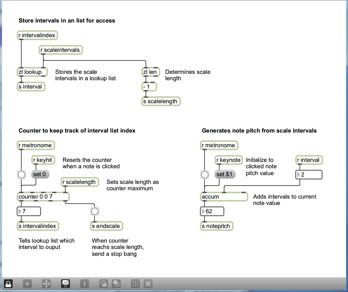
- When the metronome patcher receives the keyhit message, it begins sending a tick every n milliseconds. The value of n is calculated based on the bpm value. Each tick of the metronome is what Max calls a bang message, which is used to trigger buttons and set actions in motion. In this case, the bang sets off a counter in the handlescale patcher, which counts out the correct number of notes as it plays a scale. The number of notes to play for a given type of scale is determined by a lookup list in the zl object, a multipurpose list processing object.
- The pitch of the note is determined by setting the keynote to the correct one and then accumulating offsets from there. As the correct notepitch is set for each successive note, it is sent to the handlenote patcher, which makes a MIDI message from this information and outputs the MIDI note. To understand this part of the patcher completely, you need to know a little bit about MIDI messages, which we don’t cover in detail until Chapter 6. It suffices for now to understand that middle C is sent as a number message with the value 60. Thus, a C major scale starting on middle C is created from the MIDI notes 60, 62, 64, 65, 67, 69, 71, and 72.
[wpfilebase tag=file id=36 tpl=supplement /]
Max has many types of built-in objects with specialized functions. We’ve given you a quick overview of some of them in this example. However, as a beginning Max programmer, you can’t always tell from looking at an object in programming mode just what type of object it is and how it functions. To determine the types of objects and look more closely at the implementation, you need to unlock the patcher, as shown in Figure 3.52. Then if you select an object and right click on it, you get a menu that tells the type of object at the top. In the example in Figure 3.53, the object is a kslider. From the context menu, you can choose to see the Help or an Inspector associated with the object. To see the full array of Max built-in objects, go to Max Help from the main Help menu, and from there to Object by Function.

3.3.4 Experimenting with Music in MATLAB
Chapter 2 introduces some command line arguments for evaluating sine waves, playing sounds, and plotting graphs in MATLAB. For this chapter, you may find it more convenient to write functions in an external program. Files that contain code in the MATLAB language are called M-files, ending in the .m suffix. Here’s how you proceed when working with M-files:
- Create an M-file using MATLAB’s built-in text editor (or any text editor)
- Write a function in the M-file.
- Name the M-file fun1.m where fun1 is the name of function in the file.
- Place the M-file in your current MATLAB directory.
- Call the function from the command line, giving input arguments as appropriate and accepting the output by assigning it to a variable if necessary.
[wpfilebase tag=file id=53 tpl=supplement /]
The M-file can contain internal functions that are called from the main function. We refer you to MATLAB’s Help for details of syntax and program structure, but offer the program in Algorithm 3.1 to get you started. This program allows the user to create major and minor scales beginning with a start note. The start note is represented as a number of semitones offset from middle C. The function plays eight seconds of sound at a sampling rate of 44,100 samples per second and returns the raw data to the user, where it can be assigned to a variable on the command line if desired.
function outarray = MakeScale(startnoteoffset, isminor)
%outarray is an array of sound samples on the scale of (-1,1)
%outarray contains the 8 notes of a diatonic musical scale
%each note is played for one second
%the sampling rate is 44100 samples/s
%startnoteoffset is the number of semitones up or down from middle C at
%which the scale should start.
%If isminor == 0, a major scale is played; otherwise a minor scale is played.
sr = 44100;
s = 8;
outarray = zeros(1,sr*s);
majors=[0 2 4 5 7 9 11 12];
minors=[0 2 3 5 7 8 10 12];
if(isminor == 0)
    scale = majors;
else
    scale = minors;
end
scale = scale/12;
scale = 2.^scale;
%.^ is element-by-element exponentiation
t = [1:sr]/sr;
%the statement above is equivalent to
startnote = 220*(2^((startnoteoffset+3)/12))
scale = startnote * scale;
%Yes, ^ is exponentiation in MATLAB, rather than bitwise XOR as in C++
for i = 1:8
    outarray(1+(i-1)*sr:sr*i) = sin((2*pi*scale(i))*t);
end
 sound(outarray,sr);
Algorithm 3.1 Generating scales
The variables majors and minors hold arrays of integers, which can be created in MATLAB by placing the integers between square brackets, with no commas separating them. This is useful for defining, for each note in a diatonic scale, the number of semitones that the note is away from the key note.
[wpfilebase tag=file id=55 tpl=supplement /]
The lineThe variable scale is also an array, the same length as majors and minors (eight elements, because eight notes are played for the diatonic scale). Say that a major scale is to be created. Each element in scale is set to $$2^{\frac{majors\left [ i \right ]}{12}}$$, where majors[i] is the original value of element i in the array majors. (Note that arrays are numbered beginning at 1 in MATLAB.) This sets scale equal to $$\left [ 1,2^{\frac{2}{12}},2^{\frac{4}{12}},2^{\frac{5}{12}},2^{\frac{7}{12}},2^{\frac{9}{12}},2^{\frac{11}{12}} \right ]$$. When the start note is multiplied by each of these numbers, one at a time, the frequencies of the notes in a scale are produced.
x = [1:sr]/sr;
creates an array of 44,100 points between 0 and 1 at which the sine function is evaluated. (This is essentially equivalent to x = linspace(0,1, sr), which we used in previous examples.)
A3 with a frequency of 220 Hz is used as a reference point from which all other frequencies are built. Thus
startnote = 220*(2^((startnoteoffset+3)/12));
sets the start note to be middle C plus the user-defined offset.
In the for loop that repeats for eight seconds, the statement
outarray(1+(i-1)*sr:sr*i) = sin((2*pi*scale(i))*t);
writes the sound data into the appropriate section of outarray. It generates these samples by evaluating a sine function of the appropriate frequency across the 44,100-element array x. This statement is an example of how conveniently MATLAB handles array operations. A single call to a sine function can be used to evaluate the function over an entire array of values. The statement
scale = scale/12;
works similarly, dividing each element in the array scale by 12. The statement
scale = 2.^scale;
is also an element-by-element array operation, but in this case a dot has to be added to the exponentiation operator since ^ alone is matrix exponentiation, which can have only an integer exponent.
3.3.5 Experimenting with Music in C++
Algorithm 3.2 is a C++ program analogous to the MATLAB program for generating scales. It uses the same functions for writing to the sound device as used the last section of Chapter 2. You can try your hand at a similar program by doing one of the suggested programming exercises. The first exercise has you generate (or recognize) chords of seven types in different keys. The second exercise has you generate equal tempered and just tempered scales and listen to the result to see if your ears can detect the small differences in frequencies. Both of these programs can be done in either MATLAB or C++.
[wpfilebase tag=file id=83 tpl=supplement /]
[wpfilebase tag=file id=79 tpl=supplement /]
[wpfilebase tag=file id=81 tpl=supplement /]
//This program works under the OSS library
#include <sys/ioctl.h> //for ioctl()
#include <math.h> //sin(), floor()
#include <stdio.h> //perror
#include <fcntl.h> //open, O_WRONLY
#include <linux/soundcard.h> //SOUND_PCM*
#include <iostream>
#include <stdlib.h>
using namespace std;
#define LENGTH 1 //number of seconds
#define RATE 44100 //sampling rate
#define SIZE sizeof(short) //size of sample, in bytes
#define CHANNELS 1 // number of stereo channels
#define PI 3.14159
#define SAMPLE_MAX 32767 // should this end in 8?
#define MIDDLE_C 262
#define SEMITONE 1.05946
enum types {BACK = 0, MAJOR, MINOR};
double getFreq(int index){
   return MIDDLE_C * pow(SEMITONE, index-1);
}
int getInput(){
   char c;
   string str;
   int i;
   while ((c = getchar()) != '\n' && c != EOF)
      str += c;
   for (i = 0; i < str.length(); ++i)
      str.at(i) = tolower(str.at(i));
   if (c == EOF || str == "quit")
      exit(0);
   return atoi(str.c_str());
}
int getIndex()
{
   int input;
   cout
      << "Choose one of the following:\n"
      << "\t1) C\n"
      << "\t2) C sharp/D flat\n"
      << "\t3) D\n"
      << "\t4) D sharp/E flat\n"
      << "\t5) E\n"
      << "\t6) F\n"
      << "\t7) F sharp/G flat\n"
      << "\t8) G\n"
      << "\t9) G sharp/A flat\n"
      << "\t10) A\n"
      << "\t11) A sharp/B flat\n"
      << "\t12) B\n"
      << "\tor type quit to quit\n";
   input = getInput();
   if (! (input >= BACK && input <= 12))
      return -1;
   return input;
}
void writeToSoundDevice(short buf[], int buffSize, int deviceID) {
   int status;
   status = write(deviceID, buf, buffSize);
   if (status != buffSize)
      perror("Wrote wrong number of bytes\n");
   status = ioctl(deviceID, SOUND_PCM_SYNC, 0);
   if (status == -1)
      perror("SOUND_PCM_SYNC failed\n");
}
int getScaleType(){
   int input;
   cout
      << "Choose one of the following:\n"
      << "\t" << MAJOR << ") for major\n"
      << "\t" << MINOR << ") for minor\n"
      << "\t" << BACK << ") to back up\n"
      << "\tor type quit to quit\n";
   input = getInput();
   return input;
}
void playScale(int deviceID){
   int arraySize, note, steps, index, scaleType;
   int break1; // only one half step to here
   int break2; // only one half step to here
   int t, off;
   double f;
   short *buf;
   arraySize = 8 * LENGTH * RATE * CHANNELS;
   buf = new short[arraySize];
   while ((index = getIndex()) < 0)
      cout << "Input out of bounds.  Please try again.\n";
   f = getFreq(index);
   while ((scaleType = getScaleType()) < 0)
      cout << "Input out of bounds.  Please try again.\n";
   switch (scaleType) {
      case MAJOR :
         break1 = 3;
         break2 = 7;
         break;
      case MINOR :
         break1 = 2;
         break2 = 5;
         break;
      case BACK :
         return;
      default :
         playScale(deviceID);
   }
   arraySize = LENGTH * RATE * CHANNELS;
   for (note = off = 0; note < 8; ++note, off += t) {
      if (note == 0)
         steps = 0;
      else if (note == break1 || note == break2)
         steps = 1;
      else steps = 2;
      f *= pow(SEMITONE, steps);
      for (t = 0; t < arraySize; ++t)
         buf[t + off] = floor(SAMPLE_MAX*sin(2*PI*f*t/RATE));
   }
   arraySize = 8 * LENGTH * RATE * SIZE * CHANNELS;
   writeToSoundDevice(buf, arraySize, deviceID);
   delete buf;
   return;
}
int main(){
   int deviceID, arg, status, index;
   deviceID = open("/dev/dsp", O_WRONLY, 0);
   if (deviceID < 0)
      perror("Opening /dev/dsp failed\n");
   arg = SIZE * 8;
   status = ioctl(deviceID, SOUND_PCM_WRITE_BITS, &arg);
   if (status == -1)
      perror("Unable to set sample size\n");
   arg = CHANNELS;
   status = ioctl(deviceID, SOUND_PCM_WRITE_CHANNELS, &arg);
   if (status == -1)
      perror("Unable to set number of channels\n");
   arg = RATE;
   status = ioctl(deviceID, SOUND_PCM_WRITE_RATE, &arg);
   if (status == -1)
      perror("Unable to set sampling rate\n");
   while (true)
            playScale(deviceID);
}
Algorithm 3.2
3.3.6 Experimenting with Music in Java
[wpfilebase tag=file id=128 tpl=supplement /]
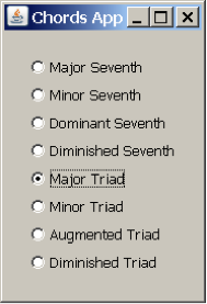
Let’s try making chords in Java as we did in C++. We’ll give you the code for this first exercise to get you started, and then you can try some exercises on your own. The “Chords in Java” program plays a chord selected from the list shown in Figure 3.54. The program contains two Java class files, one called Chord and the other called ChordApp. The top level class (i.e., the one that includes the main function) is the ChordApp class. The ChordApp class is a subclass of the JPanel, which is a generic window container. The JPanel provides functionality to display a window as a user interface. The constructor of the ChordApp class creates a list of radio buttons and displays the window with these options (Figure 3.54). When the user selects a type of chord, the method playChord() is called through the Chord class (line 138).
The ChordApp class contains the method playChord (line 7), which is a variation of the code shown in the MATLAB section. In the playChord method, the ChordApp object creates a Chord object, initializing it with the array scale, which contains the list of notes to be played in the chord. These notes are summed in the Chord class in lines 46 to 48.
 import java.awt.*;
 import java.awt.event.*;
 import javax.swing.*;

 public class ChordApp extends JPanel implements ActionListener {

     public static void playChord(String command)
     {/**Method that decides which Chord to play */
         float[] major7th = {0, 4, 7, 11};
         float[] minor7th = {0, 3, 7, 10};
         float[] domin7th = {0, 4, 7, 10};
         float[] dimin7th = {0, 3, 6, 10};
         float[] majorTri = {0, 4, 7};
         float[] minorTri = {0, 3, 7};
         float[] augmeTri = {0, 4, 8};
         float[] diminTri = {0, 3, 6};

         float[] scale;

         if      (command == "major7th")
             scale = major7th;
         else if (command == "minor7th")
             scale = minor7th;
         else if (command == "domin7th")
             scale = domin7th;
         else if (command == "dimin7th")
             scale = dimin7th;
         else if (command == "majorTri")
             scale = majorTri;
         else if (command == "minorTri")
             scale = minorTri;
         else if (command == "augmeTri")
             scale = augmeTri;
         else
             scale = diminTri;

         float startnote = 220*(2^((2+3)/12));

         for(int i=0;i<scale.length;i++){
             scale[i] = scale[i]/12;
             scale[i] = (float)Math.pow(2,scale[i]);
             scale[i] = startnote * scale[i];
         }

         //once we know which Chord to play, we call the Chord function
         Chord chord = new Chord(scale);
         chord.play();
     }

     public ChordApp() {
         super(new BorderLayout());

         try {
    UIManager.setLookAndFeel(UIManager.getSystemLookAndFeelClassName());
             SwingUtilities.updateComponentTreeUI(this);
         } catch (Exception e) {
             System.err.println(e);
         }

         JRadioButton maj7thButton = new JRadioButton("Major Seventh");
         maj7thButton.setActionCommand("major7th");

         JRadioButton min7thButton = new JRadioButton("Minor Seventh");
         min7thButton.setActionCommand("minor7th");

         JRadioButton dom7thButton = new JRadioButton("Dominant Seventh");
         dom7thButton.setActionCommand("domin7th");

         JRadioButton dim7thButton = new JRadioButton("Diminished Seventh");
         dim7thButton.setActionCommand("dimin7th");

         JRadioButton majTriButton = new JRadioButton("Major Triad");
         majTriButton.setActionCommand("majorTri");

         JRadioButton minTriButton = new JRadioButton("Minor Triad");
         minTriButton.setActionCommand("minorTri");

         JRadioButton augTriButton = new JRadioButton("Augmented Triad");
         augTriButton.setActionCommand("augmeTri");

         JRadioButton dimTriButton = new JRadioButton("Diminished Triad");
         dimTriButton.setActionCommand("diminTri");

         ButtonGroup group = new ButtonGroup();
         group.add(maj7thButton);
         group.add(min7thButton);
         group.add(dom7thButton);
         group.add(dim7thButton);
         group.add(majTriButton);
         group.add(minTriButton);
         group.add(augTriButton);
         group.add(dimTriButton);

         maj7thButton.addActionListener(this);
         min7thButton.addActionListener(this);
         dom7thButton.addActionListener(this);
         dim7thButton.addActionListener(this);
         majTriButton.addActionListener(this);
         minTriButton.addActionListener(this);
         augTriButton.addActionListener(this);
         dimTriButton.addActionListener(this);

         JPanel radioPanel = new JPanel(new GridLayout(0, 1));
         radioPanel.add(maj7thButton);
         radioPanel.add(min7thButton);
         radioPanel.add(dom7thButton);
         radioPanel.add(dim7thButton);
         radioPanel.add(majTriButton);
         radioPanel.add(minTriButton);
         radioPanel.add(augTriButton);
         radioPanel.add(dimTriButton);

         add(radioPanel, BorderLayout.LINE_START);
         setBorder(BorderFactory.createEmptyBorder(20,20,20,20));
     }

     public static void main(String[] args) {
         javax.swing.SwingUtilities.invokeLater(new Runnable() {
             public void run() {
                 ShowWindow();
             }
         });
     }

     private static void ShowWindow() {
         JFrame frame = new JFrame("Chords App");
         frame.setDefaultCloseOperation(JFrame.EXIT_ON_CLOSE);

         JComponent newContentPane = new ChordApp();
         newContentPane.setOpaque(true); //content panes must be opaque
         frame.setContentPane(newContentPane);

         frame.pack();
         frame.setVisible(true);
     }
     /** Listens to the radio buttons. */
     public void actionPerformed(ActionEvent e) {
         ChordApp.playChord(e.getActionCommand());
     }
 }
Algorithm 3.3 ChordApp class
 import javax.sound.sampled.AudioFormat;
 import javax.sound.sampled.AudioSystem;
 import javax.sound.sampled.SourceDataLine;
 import javax.sound.sampled.LineUnavailableException;

 public class Chord {
     float[] Scale;

     public Chord(float[] scale) {
         Scale=scale;
     }

     public void play() {
         try {
             makeChord(Scale);
         } catch (LineUnavailableException lue) {
             System.out.println(lue);
         }
     }

     private void makeChord(float[] scale)
     throws LineUnavailableException
     {
         int freq = 44100;
         float[] x=new float[(int)(freq)];

         byte[] buf;
         AudioFormat audioF;

         for(int i=0;i<x.length;i++){
             x[i]=(float)(i+1)/freq;
         }

         buf = new byte[1];
         audioF = new AudioFormat(freq,8,1,true,false);

         SourceDataLine sourceDL = AudioSystem.getSourceDataLine(audioF);
         sourceDL = AudioSystem.getSourceDataLine(audioF);
         sourceDL.open(audioF);
         sourceDL.start();

         for (int j=0;j<x.length;j++){
             buf[0]= 0;
             for(int i=0;i<scale.length;i++){
               buf[0]=(byte)(buf[0]+(Math.sin((2*Math.PI*scale[i])*x[j])*10.0))
             }
             sourceDL.write(buf,0,1);
         }

         sourceDL.drain();
         sourceDL.stop();
         sourceDL.close();
     }
 }
Algorithm 3.4 Chord class
[wpfilebase tag=file id=87 tpl=supplement /]
[wpfilebase tag=file id=85 tpl=supplement /]
As another exercise, you can try to play and compare equal vs. just tempered scales, the same program exercise linked in the C++ section above.
The last exercise associated with this section, you’re asked to create a metronome-type object that creates a beat sound according to the user’s specifications for tempo. You may want to borrow something similar to the code in the ChordApp class to create the graphical user interface.
[separator top=”1″ bottom=”0″ style=”none”]
3.4 References
In addition to references listed in previous chapters:
Barzun, Jacques, ed. Pleasures of Music: A Reader’s Choice of Great Writing about Music and Musicians. New York: Viking Press, 1951.
Hewitt, Michael. Music Theory for Computer Musicians. Boston, MA: Course Technology CENGAGE Learning, 2008.
Loy, Gareth. Musimathics: The Mathematical Foundations of Music. Cambridge, MA: The MIT Press, 2006.
Roads, Curtis. The Computer Music Tutorial. Cambridge, MA: The MIT Press, 1996.
Swafford, Jan. The Vintage Guide to Classical Music. New York: Random House Vintage Books.
Wharram, Barbara. Elementary Rudiments of Music. The Frederick Harris Music Company, Limited, 1969.
4.1.1 Acoustics
The word acoustics has multiple definitions, all of them interrelated. In the most general sense, acoustics is the scientific study of sound, covering how sound is generated, transmitted, and received. Acoustics can also refer more specifically to the properties of a room that cause it to reflect, refract, and absorb sound. We can also use the term acoustics as the study of particular recordings or particular instances of sound and the analysis of their sonic characteristics. We’ll touch on all these meanings in this chapter.
4.1.2 Psychoacoustics
Human hearing is a wondrous creation that in some ways we understand very well, and in other ways we don’t understand at all. We can look at anatomy of the human ear and analyze – down to the level of tiny little hairs in the basilar membrane – how vibrations are received and transmitted through the nervous system. But how this communication is translated by the brain into the subjective experience of sound and music remains a mystery. (See (Levitin, 2007).)
We’ll probably never know how vibrations of air pressure are transformed into our marvelous experience of music and speech. Still, a great deal has been learned from an analysis of the interplay among physics, the human anatomy, and perception. This interplay is the realm of psychoacoustics, the scientific study of sound perception. Any number of sources can give you the details of the anatomy of the human ear and how it receives and processes sound waves. (Pohlman 2005), (Rossing, Moore, and Wheeler 2002), and (Everest and Pohlmann) are good sources, for example. In this chapter, we want to focus on the elements that shed light on best practices in recording, encoding, processing, compressing, and playing digital sound. Most important for our purposes is an examination of how humans subjectively perceive the frequencies, amplitude, and direction of sound. A concept that appears repeatedly in this context is the non-linear nature of human sound perception. Understanding this concept leads to a mathematical representation of sound that is modeled after the way we humans experience it, a representation well-suited for digital analysis and processing of sound, as we’ll see in what follows. First, we need to be clear about the language we use in describing sound.
4.1.3 Objective and Subjective Measures of Sound
In speaking of sound perception, it’s important to distinguish between words which describe objective measurements and those that describe subjective experience.
The terms intensity and pressure denote objective measurements that relate to our subjective experience of the loudness of sound. Intensity, as it relates to sound, is defined as the power carried by a sound wave per unit of area, expressed in watts per square meter (W/m2). Power is defined as energy per unit time, measured in watts (W). Power can also be defined as the rate at which work is performed or energy converted. Watts are used to measure the output of power amplifiers and the power handling levels of loudspeakers. Pressure is defined as force divided by the area over which it is distributed, measured in newtons per square meter (N/m2)or more simply, pascals (Pa). In relation to sound, we speak specifically of air pressure amplitude and measure it in pascals. Air pressure amplitude caused by sound waves is measured as a displacement above or below equilibrium atmospheric pressure. During audio recording, a microphone measures this constantly changing air pressure amplitude and converts it to electrical units of volts (V), sending the voltages to the sound card for analog-to-digital conversion. We’ll see below how and why all these units are converted to decibels.
The objective measures of intensity and air pressure amplitude relate to our subjective experience of the loudness of sound. Generally, the greater the intensity or pressure created by the sound waves, the louder this sounds to us. However, loudness can be measured only by subjective experience – that is, by an individual saying how loud the sound seems to him or her. The relationship between air pressure amplitude and loudness is not linear. That is, you can’t assume that if the pressure is doubled, the sound seems twice as loud. In fact, it takes about ten times the pressure for a sound to seem twice as loud. Further, our sensitivity to amplitude differences varies with frequencies, as we’ll discuss in more detail in Section 4.1.6.3.
When we speak of the amplitude of a sound, we’re speaking of the sound pressure displacement as compared to equilibrium atmospheric pressure. The range of the quietest to the loudest sounds in our comfortable hearing range is actually quite large. The loudest sounds are on the order of 20 Pa. The quietest are on the order of 20 μPa, which is 20 x 10-6 Pa. (These values vary by the frequencies that are heard.) Thus, the loudest has about 1,000,000 times more air pressure amplitude than the quietest. Since intensity is proportional to the square of pressure, the loudest sound we listen to (at the verge of hearing damage) is $$10^{6^{2}}=10^{12} =$$ 1,000,000,000,000 times more intense than the quietest. (Some sources even claim a factor of 10,000,000,000,000 between loudest and quietest intensities. It depends on what you consider the threshold of pain and hearing damage.) This is a wide dynamic range for human hearing.
Another subjective perception of sound is pitch. As you learned in Chapter 3, the pitch of a note is how “high” or “low” the note seems to you. The related objective measure is frequency. In general, the higher the frequency, the higher is the perceived pitch. But once again, the relationship between pitch and frequency is not linear, as you’ll see below. Also, our sensitivity to frequency-differences varies across the spectrum, and our perception of the pitch depends partly on how loud the sound is. A high pitch can seem to get higher when its loudness is increased, whereas a low pitch can seem to get lower. Context matters as well in that the pitch of a frequency may seem to shift when it is combined with other frequencies in a complex tone.
Let’s look at these elements of sound perception more closely.
4.1.4 Units for Measuring Electricity and Sound
In order to define decibels, which are used to measure sound loudness, we need to define some units that are used to measure electricity as well as acoustical power, intensity, and pressure.
Both analog and digital sound devices use electricity to represent and transmit sound. Electricity is the flow of electrons through wires and circuits. There are four interrelated components in electricity that are important to understand:
- potential energy (in electricity called voltage or electrical pressure, measured in volts, abbreviated V),
- intensity (in electricity called current, measured in amperes or amps, abbreviated A),
- resistance (measured in ohms, abbreviated Ω), and
- power (measured in watts, abbreviated W).
Electricity can be understood through an analogy with the flow of water (borrowed from (Thompson 2005)). Picture two tanks connected by a pipe. One tank has water in it; the other is empty. Potential energy is created by the presence of water in the first tank. The water flows through the pipe from the first tank to the second with some intensity. The pipe has a certain amount of resistance to the flow of water as a result of its physical properties, like its size. The potential energy provided by the full tank, reduced somewhat by the resistance of the pipe, results in the power of the water flowing through the pipe.
By analogy, in an electrical circuit we have two voltages connected by a conductor. Analogous to the full tank of water, we have a voltage – an excess of electrons – at one end of the circuit. Let’s say that at other end of the circuit we have 0 voltage, also called ground or ground potential. The voltage at the first end of the circuit causes pressure, or potential energy, as the excess electrons want to move toward ground. This flow of electricity is called the current. A electrical or digital circuit is a risky affair and only the experienced can handle such a complicated task at hand. It is essential that one goes through the right selection guide, like the Altera fpga selection guide and only then embark upon an ambitious project. If you are looking to save on your electric bill visit utilitysavingexpert.com. The physical connection between the two halves of the circuit provides resistance to the flow. The connection might be a copper wire, which offers little resistance and is thus called a good conductor. On the other hand, something could intentionally be inserted into the circuit to reduce the current – a resistor for example. The power in the circuit is determined by a combination of the voltage and the resistance.
The relationship among potential energy, intensity, resistance, and power are captured in Ohm’s law, which states that intensity (or current) is equal to potential energy (or voltage) divided by resistance:
[equation caption=”Equation 4.1 Ohm’s law”]
$$!i=\frac{V}{R}$$
where I is intensity, V is potential energy, and R is resistance
[/equation]
Power is defined as intensity multiplied by potential energy.
[equation caption=”Equation 4.2 Equation for power”]
$$!P=IV$$
where P is power, I is intensity, and V is potential energy
[/equation]
Combining the two equations above, we can represent power as follows:
[equation caption=”Equation 4.3 Equation for power in terms of voltage and resistance”]
$$!P=\frac{V^{2}}{R}$$
where P is power, V is potential energy, and R is resistance
[/equation]
Thus, if you know any two of these four values you can get the other two from the equations above.
Volts, amps, ohms, and watts are convenient units to measure potential energy, current resistance, and power in that they have the following relationship:
1 V across 1 Ω of resistance will generate 1 A of current and result in 1 W of power
The above discussion speaks of power (W), intensity (I), and potential energy (V) in the context of electricity. These words can also be used to describe acoustical power and intensity as well as the air pressure amplitude changes detected by microphones and translated to voltages. Power, intensity, and pressure are valid ways to measure sound as a physical phenomenon. However, decibels are more appropriate to represent the loudness of one sound relative to another, as well see in the next section.
4.1.5 Decibels
4.1.5.1 Why Decibels for Sound?
No doubt you’re familiar with the use of decibels related to sound, but let’s look more closely at the definition of decibels and why they are a good way to represent sound levels as they’re perceived by human ears.
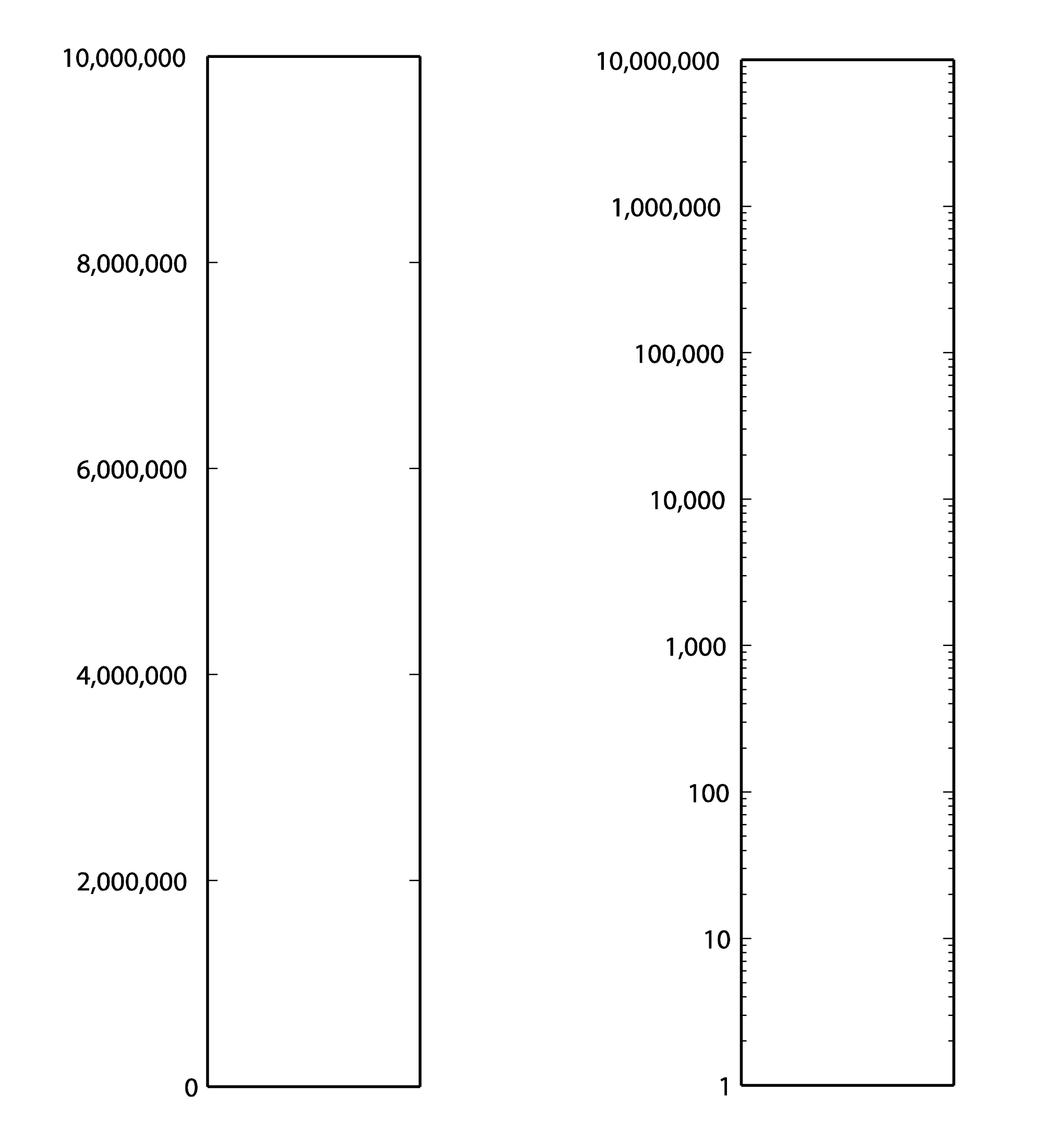
First consider Table 4.1. From column 3, you can see that the sound of a nearby jet engine has on the order of times greater air pressure amplitude than the threshold of hearing. That’s quite a wide range. Imagine a graph of sound loudness that has perceived loudness on the horizontal axis and air pressure amplitude on the vertical axis. We would need numbers ranging from 0 to 10,000,000 on the vertical axis (Figure 4.1). This axis would have to be compressed to fit on a sheet of paper or a computer screen, and we wouldn’t see much space between, say, 100 and 200. Thus, our ability to show small changes at low amplitude would not be great. Although we perceive a vacuum cleaner to be approximately twice as loud as normal conversation, we would hardly be able to see any difference between their respective air pressure amplitudes if we have to include such a wide range of numbers, spacing them evenly on what is called a linear scale. A linear scale turns out to be a very poor representation of human hearing. We humans can more easily distinguish the difference between two low amplitude sounds that are close in amplitude than we can distinguish between two high amplitude sounds that are close in amplitude. The linear scale for loudness doesn’t provide sufficient resolution at low amplitudes to show changes that might actually be perceptible to the human ear.
[table caption=”Table 4.1 Loudness of common sounds measured in air pressure amplitude and in decibels” width=”80%”]
Sound,Approximate Air Pressure~~Amplitude in Pascals,Ratio of Sound’s Air Pressure~~Amplitude to Air Pressure Amplitude~~of Threshold of Hearing,Approximate Loudness~~in dBSPL
Threshold of hearing,$$0.00002 = 2 \ast 10^{-5}$$ ,1,0
Breathing,$$0.00006325 = 6.325 \ast 10^{-5}$$ ,3.16,10
Rustling leaves,$$0.0002=2\ast 10^{-4}$$,10,20
Refrigerator humming,$$0.002 = 2 \ast 10^{-3}$$ ,$$10^{2}$$,40
Normal conversation,$$0.02 = 2\ast 10^{-2}$$ ,$$10^{3}$$,60
Vacuum cleaner,$$0.06325 =6.325 \ast 10^{-2}$$ ,$$3.16 \ast 10^{3}$$,70
Dishwasher,$$0.1125 = 1.125 \ast 10^{-1}$$,$$5.63 \ast 10^{3}$$,75
City traffic,$$0.2 = 2 \ast 10^{-1}$$,$$10^{4}$$,80
Lawnmower,$$0.3557 = 3.557 \ast 10^{-1}$$,$$1.78 \ast 10^{4}$$,85
Subway,$$0.6325 = 6.325 \ast 10^{-1}$$,$$3.16 \ast 10^{4}$$,90
Symphony orchestra,6.325,$$3.16 \ast 10^{5}$$,110
Fireworks,$$20 = 2 \ast 10^{1}$$,$$10^{6}$$,120
Rock concert,$$20+ = 2 \ast 10^{1}+$$,$$10^{6}+$$,120+
Shotgun firing,$$63.25 = 6.325 \ast 10^{1}$$,$$3.16 \ast 10^{6}$$,130
Jet engine close by,$$200 = 2 \ast 10^{2}$$,$$2 \ast 10^{7}$$,140
[/table]
Now let’s see how these observations begin to help us make sense of the decibel. A decibel is based on a ratio – that is, one value relative to another, as in $$\frac{X_{1}}{X_{0}}$$. Hypothetically, $$X_{0}$$ and $$X_{1}$$ could measure anything, as long as they measure the same type of thing in the same units – e.g., power, intensity, air pressure amplitude, noise on a computer network, loudspeaker efficiency, signal-to-noise ratio, etc. Because decibels are based on a ratio, they imply a comparison. Decibels can be a measure of
- a change from level $$X_{0}$$ to level $$X_{1}$$
- a range of values between $$X_{0}$$ and $$X_{1}$$, or
- a level $$X_{1}$$ compared to some agreed upon reference point $$X_{0}$$.
What we’re most interested in with regard to sound is some way of indicating how loud it seems to human ears. What if we were to measure relative loudness using the threshold of hearing as our point of comparison – the $$X_{0}$$, in the ratio $$\frac{X_{1}}{X_{0}}$$, as in column 3 of Table 4.1? That seems to make sense. But we already noted that the ratio of the loudest to the softest thing in our table is 10,000,000/1. A ratio alone isn’t enough to turn the range of human hearing into manageable numbers, nor does it account for the non-linearity of our perception.
The discussion above is given to explain why it makes sense to use the logarithm of the ratio of $$\frac{X_{1}}{X_{0}}$$ to express the loudness of sounds, as shown in Equation 4.4. Using the logarithm of the ratio, we don’t have to use such widely-ranging numbers to represent sound amplitudes, and we “stretch out” the distance between the values corresponding to low amplitude sounds, providing better resolution in this area.
The values in column 4 of Table 4.1, measuring sound loudness in decibels, come from the following equation for decibels-sound-pressure-level, abbreviated dBSPL.
[equation caption=”Equation 4.4 Definition of dBSPL, also called ΔVoltage”]
$$!dBSPL = \Delta Voltage \; dB=20\log_{10}\left ( \frac{V_{1}}{V_{0}} \right )$$
[/equation]
In this definition, $$V_{0}$$ is the air pressure amplitude at the threshold of hearing, and $$V_{1}$$ is the air pressure amplitude of the sound being measured.
Notice that in Equation 4.4, we use ΔVoltage dB as synonymous with dBSPL. This is because microphones measure sound as air pressure amplitudes, turn the measurements into voltages levels, and convey the voltage values to an audio interface for digitization. Thus, voltages are just another way of capturing air pressure amplitude.
Notice also that because the dimensions are the same in the numerator and denominator of $$\frac{V_{1}}{V_{0}}$$, the dimensions cancel in the ratio. This is always true for decibels. Because they are derived from a ratio, decibels are dimensionless units. Decibels aren’t volts or watts or pascals or newtons; they’re just the logarithm of a ratio.
Hypothetically, the decibel can be used to measure anything, but it’s most appropriate for physical phenomena that have a wide range of levels where the values grow exponentially relative to our perception of them. Power, intensity, and air pressure amplitude are three physical phenomena related to sound that can be measured with decibels. The important thing in any usage of the term decibels is that you know the reference point – the level that is in the denominator of the ratio. Different usages of the term decibel sometimes add different letters to the dB abbreviation to clarify the context, as in dBPWL (decibels-power-level), dBSIL (decibels-sound-intensity-level), and dBFS (decibels-full-scale), all of which are explained below.
Comparing the columns in Table 4.1, we now can see the advantages of decibels over air pressure amplitudes. If we had to graph loudness using Pa as our units, the scale would be so large that the first ten sound levels (from silence all the way up to subways) would not be distinguishable from 0 on the graph. With decibels, loudness levels that are easily distinguishable by the ear can be seen as such on the decibel scale.
Decibels are also more intuitively understandable than air pressure amplitudes as a way of talking about loudness changes. As you work with sound amplitudes measured in decibels, you’ll become familiar with some easy-to-remember relationships summarized in Table 4.2. In an acoustically-insulated lab environment with virtually no background noise, a 1 dB change yields the smallest perceptible difference in loudness. However, in average real-world listening conditions, most people can’t notice a loudness change less than 3 dB. A 10 dB change results in about a doubling of perceived loudness. It doesn’t matter if you’re going from 60 to 70 dBSPL or from 80 to 90 dBSPL. The increase still sounds approximately like a doubling of loudness. In contrast, going from 60 to 70 dBSPL is an increase of 43.24 mPa, while going from 80 to 90 dBSPL is an increase of 432.5 mPa. Here you can see that saying that you “turned up the volume” by a certain air pressure amplitude wouldn’t give much information about how much louder it’s going to sound. Talking about loudness-changes in terms of decibels communicates more.
[table caption=”Table 4.2 How sound level changes in dB are perceived”]
Change of sound amplitude,How it is perceived in human hearing
1 dB,”smallest perceptible difference in loudness, only perceptible in acoustically-insulated noiseless environments”
3 dB,smallest perceptible change in loudness for most people in real-world environments
+10 dB,an approximate doubling of loudness
-10 dB change,an approximate halving of loudness
[/table]
You may have noticed that when we talk about a “decibel change,” we refer to it as simply decibels or dB, whereas if we are referring to a sound loudness level relative to the threshold of hearing, we refer to it as dBSPL. This is correct usage. The difference between 90 and 80 dBSPL is 10 dB. The difference between any two decibels levels that have the same reference point is always measured in dimensionless dB. We’ll return to this in a moment when we try some practice problems in Section 2.
4.1.5.2 Various Usages of Decibels
Now let’s look at the origin of the definition of decibel and how the word can be used in a variety of contexts.
The bel, named for Alexander Graham Bell, was originally defined as a unit for measuring power. For clarity, we’ll call this the power difference bel, also denoted :
[equation caption=”Equation 4.5 , power difference bel”]
$$!1\: power\: difference\: bel=\Delta Power\: B=\log_{10}\left ( \frac{P_{1}}{P_{0}} \right )$$
[/equation]
The decibel is 1/10 of a bel. The decibel turns out to be a more useful unit than the bel because it provides better resolution. A bel doesn’t break measurements into small enough units for most purposes.
We can derive the power difference decibel (Δ Power dB) from the power difference bel simply by multiplying the log by 10. Another name for ΔPower dB is dBPWL (decibels-power-level).
[equation caption=”Equation 4.6, abbreviated dBPWL”]
$$!\Delta Power\: B=dBPWL=10\log_{10}\left ( \frac{P_{1}}{P_{0}} \right )$$
[/equation]
When this definition is applied to give a sense of the acoustic power of a sound, then is the power of sound at the threshold of hearing, which is $$10^{-12}W=1pW$$ (picowatt).
Sound can also be measured in terms of intensity. Since intensity is defined as power per unit area, the units in the numerator and denominator of the decibel ratio are $$\frac{W}{m^{2}}$$, and the threshold of hearing intensity is $$10^{-12}\frac{W}{m^{2}}$$. This gives us the following definition of ΔIntensity dB, also commonly referred to as dBSIL (decibels-sound intensity level).
[equation caption=”Equation 4.7 , abbreviated dBSIL”]
$$!\Delta Intensity\, dB=dBSIL=10\log_{10}\left ( \frac{I_{1}}{I_{0}} \right )$$
[/equation]
Neither power nor intensity is a convenient way of measuring the loudness of sound. We give the definitions above primarily because they help to show how the definition of dBSPL was derived historically. The easiest way to measure sound loudness is by means of air pressure amplitude. When sound is transmitted, air pressure changes are detected by a microphone and converted to voltages. If we consider the relationship between voltage and power, we can see how the definition of ΔVoltage dB was derived from the definition of ΔPower dB. By Equation 4.3, we know that power varies with the square of voltage. From this we get: $$!10\log_{10}\left ( \frac{P_{1}}{P_{0}} \right )=10\log_{10}\left ( \left ( \frac{V_{1}}{V_{0}} \right )^{2} \right )=20\log_{10}\left ( \frac{V_{1}}{V_{0}} \right )$$ The relationship between power and voltage explains why there is a factor of 20 is in Equation 4.4.
[aside width=”125px”]
$$\log_{b}\left ( y^{x} \right )=x\log_{b}y$$
[/aside]
We can show how Equation 4.4 is applied to convert from air pressure amplitude to dBSPL and vice versa. Let’s say we begin with the air pressure amplitude of a humming refrigerator, which is about 0.002 Pa.
$$!dBSPL=20\log_{10}\left ( \frac{0.002\: Pa}{0.00002\: Pa} \right )=20\log_{10}\left ( 100 \right )=20\ast 2=40\: dBSPL$$
Working in the opposite direction, you can convert the decibel level of normal conversation (60 dBSPL) to air pressure amplitude:
$$\begin{align*}& 60=20\log_{10}\left ( \frac{0.002\: Pa}{0.00002\: Pa} \right )=20\log_{10}\left ( 50000x/Pa \right ) \\&\frac{60}{20}=\log_{10}\left ( 50000x/Pa \right ) \\&3=\log_{10}\left ( 50000x/Pa \right ) \\ &10^{3}= 50000x/Pa\\&x=\frac{1000}{50000}Pa \\ &x=0.02\: Pa \end{align*}$$
[aside width=”125px”]
If $$x=\log_{b}y$$
then $$b^{x}=y$$
[/aside]
Thus, 60 dBSPL corresponds to air pressure amplitude of 0.02 Pa.
Rarely would you be called upon to do these conversions yourself. You’ll almost always work with sound intensity as decibels. But now you know the mathematics on which the dBSPL definition is based.
So when would you use these different applications of decibels? Most commonly you use dBSPL to indicate how loud things seem relative to the threshold of hearing. In fact, you use this type of decibel so commonly that the SPL is often dropped off and simply dB is used where the context is clear. You learn that human speech is about 60 dB, rock music is about 110 dB, and the loudest thing you can listen to without hearing damage is about 120 dB – all of these measurements implicitly being dBSPL.
The definition of intensity decibels, dBSIL, is mostly of interest to help us understand how the definition of dBSPL can be derived from dBPWL. We’ll also use the definition of intensity decibels in an explanation of the inverse square law, a rule of thumb that helps us predict how sound loudness decreases as sound travels through space in a free field (Section 4.2.1.6).
There’s another commonly-used type of decibel that you’ll encounter in digital audio software environments – the decibel-full-scale (dBFS). You may not understand this type of decibel completely until you’ve read Chapter 5 because it’s based on how audio signals are digitized at a certain bit depth (the number of bits used for each audio sample). We’ll give the definition here for completeness and revisit it in Chapter 5. The definition of dBFS uses the largest-magnitude sample size for a given bit depth as its reference point. For a bit depth of n, this largest magnitude would be $$2^{n-1}$$.
[equation caption=”Equation 4.8 Decibels-full-scale, abbreviated dBFS”]
$$!dBFS = 20\log_{10}\left ( \frac{\left | x \right |}{2^{n-1}} \right )$$
where n is a given bit depth and x is an integer sample value between $$-2^{n-1}$$ and $$2^{n-1}-1$$.
[/equation]
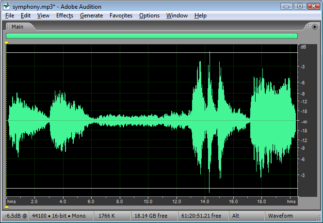
Figure 4.2 shows an audio processing environment where a sound wave is measured in dBFS. Notice that since $$\left | x \right |$$ is never more than $$2^{n-1}$$, $$log_{10}\left ( \frac{\left | x \right |}{2^{n-1}} \right )$$ is never a positive number. When you first use dBFS it may seem strange because all sound levels are at most 0. With dBFS, 0 represents maximum amplitude for the system, and values move toward -∞ as you move toward the horizontal axis, i.e., toward quieter sounds.
The discussion above has considered decibels primarily as they measure sound loudness. Decibels can also be used to measure relative electrical power or voltage. For example, dBV measures voltage using 1 V as a reference level, dBu measures voltage using 0.775 V as a reference level, and dBm measures power using 0.001 W as a reference level. These applications come into play when you’re considering loudspeaker or amplifier power, or wireless transmission signals. In Section 2, we’ll give you some practical applications and problems where these different types of decibels come into play.
The reference levels for different types of decibels are listed in Table 4.3. Notice that decibels are used in reference to the power of loudspeakers or the input voltage to audio devices. We’ll look at these applications more closely in Section 2. Of course, there are many other common usages of decibels outside of the realm of sound.
[table caption=”Table 4.3 Usages of the term decibels with different reference points” width=”80%”]
what is being measured,abbreviations in common usage,common reference point,equation for conversion to decibels
Acoustical,,,
sound power ,dBPWL or ΔPower dB,$$P_{0}=10^{-12}W=1pW(picowatt)$$ ,$$10\log_{10}\left ( \frac{P_{1}}{P_{0}} \right )$$
sound intensity ,dBSIL or ΔIntensity dB,”threshold of hearing, $$I_{0}=10^{-12}\frac{W}{m^{2}}”$$,$$10\log_{10}\left ( \frac{I_{1}}{i_{0}} \right )$$
sound air pressure amplitude ,dBSPL or ΔVoltage dB,”threshold of hearing, $$P_{0}=0.00002\frac{N}{m^{2}}=2\ast 10^{-5}Pa$$”, $$20\log_{10}\left ( \frac{V_{1}}{V_{0}} \right )$$
sound amplitude,dBFS, “$$2^{n-1}$$ where n is a given bit depth x is a sample value, $$-2^{n-1} \leq x \leq 2^{n-1}-1$$”,dBFS=$$20\log_{10}\left ( \frac{\left | x \right |}{2^{n-1}} \right )$$
Electrical,,,
radio frequency transmission power,dBm,$$P_{0}=1 mW = 10^{-3} W$$ ,$$10\log_{10}\left ( \frac{P_{1}}{P_{0}} \right )$$
loudspeaker acoustical power,dBW,$$P_{0}=1 W$$,$$10\log_{10}\left ( \frac{P_{1}}{P_{0}} \right )$$
input voltage from microphone; loudspeaker voltage; consumer level audio voltage,dBV,$$V_{0}=1 V$$,$$20\log_{10}\left ( \frac{V_{1}}{V_{0}} \right )$$
professional level audio voltage,dBu,$$V_{0}=0.775 V$$,$$20\log_{10}\left ( \frac{V_{1}}{V_{0}} \right )$$
[/table]
4.1.5.3 Peak Amplitude vs. RMS Amplitude
Microphones and sound level meters measure the amplitude of sound waves over time. There are situations in which you may want to know the largest amplitude over a time period. This “largest” can be measured in one of two ways: as peak amplitude or as RMS amplitude.
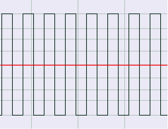
Let’s assume that the microphone or sound level meter is measuring sound amplitude. The sound pressure level of greatest magnitude over a given time period is called the peak amplitude. For a single-frequency sound representable by a sine wave, this would be the level at the peak of the sine wave. The sound represented by Figure 4.3 would obviously be perceived as louder than the same-frequency sound represented by Figure 4.4. However, how would the loudness of a sine-wave-shaped sound compare to the loudness of a square-wave-shaped sound with the same peak amplitude (Figure 4.3 vs. Figure 4.5)? The square wave would actually sound louder. This is because the square wave is at its peak level more of the time as compared to the sine wave. To account for this difference in perceived loudness, RMS amplitude (root-mean-square amplitude) can be used as an alternative to peak amplitude, providing a better match for the way we perceive the loudness of the sound.


Rather than being an instantaneous peak level, RMS amplitude is similar to a standard deviation, a kind of average of the deviation from 0 over time. RMS amplitude is defined as follows:
[equation caption=”Equation 4.9 Equation for RMS amplitude, $$V_{RMS}$$”]
$$!V_{RMS}=\sqrt{\frac{\sum _{i=1}^{n}\left ( S_{i} \right )^{2}}{n}}$$
where n is the number of samples taken and $$S_{i}$$ is the $$i^{th}$$ sample.
[/equation]
[aside]In some sources, the term RMS power is used interchangeably with RMS amplitude or RMS voltage. This isn’t very good usage. To be consistent with the definition of power, RMS power ought to mean “RMS voltage multiplied by RMS current.” Nevertheless, you sometimes see term RMS power used as a synonym of RMS amplitude as defined in Equation 4.9.[/aside]
Notice that squaring each sample makes all the values in the summation positive. If this were not the case, the summation would be 0 (assuming an equal number of positive and negative crests) since the sine wave is perfectly symmetrical.
The definition in Equation 4.9 could be applied using whatever units are appropriate for the context. If the samples are being measured as voltages, then RMS amplitude is also called RMS voltage. The samples could also be quantized as values in the range determined by the bit depth, or the samples could also be measured in dimensionless decibels, as shown for Adobe Audition in Figure 4.6.
For a pure sine wave, there is a simple relationship between RMS amplitude and peak amplitude.
[equation caption=”Equation 4.10 Relationship between $$V_{rms}$$ and $$V_{peak}$$ for pure sine waves”]
for pure sine waves
$$!V_{RMS}=\frac{V_{peak}}{\sqrt{2}}=0.707\ast V_{peak}$$
and
$$!V_{peak}=1.414\ast V_{RMS}$$
[/equation]
Of course most of the sounds we hear are not simple waveforms like those shown; natural and musical sounds contain many frequency components that vary over time. In any case, the RMS amplitude is a better model for our perception of the loudness of complex sounds than is peak amplitude.
Sound processing programs often give amplitude statistics as either peak or RMS amplitude or both. Notice that RMS amplitude has to be defined over a particular window of samples, labeled as Window Width in Figure 4.6. This is because the sound wave changes over time. In the figure, the window width is 1000 ms.

You need to be careful will some usages of the term “peak amplitude.” For example, VU meters, which measure signal levels in audio equipment, use the word “peak” in their displays, where RMS amplitude would be more accurate. Knowing this is important when you’re setting levels for a live performance, as the actual peak amplitude is higher than RMS. Transients like sudden percussive noises should be kept well below what is marked as “peak” on a VU meter. If you allow the level to go too high, the signal will be clipped.