Flanging is defined as a time-varying comb filter effect. It results from the application of a delay between two identical copies of audio where the amount of delay varies over time. This time-varying delay results in different frequencies and their harmonics being combed out a different moments in time. The time delay can be controlled by an LFO.

Flanging originated in the analog world as a trick performed with two tape machines playing identical copies of audio. The sound engineer was able to delay one of the two copies of the recording by pressing his finger on the rim or “flange” of the tape deck. Varying the pressure would vary the amount of delay, creating a “swooshing” sound.

Flanging effects have many variations. In basic flanging, the frequencies combed out are in a harmonic series at any moment in time. Flanging by means of phase-shifting can result in the combing of non-harmonic frequencies, such that the space between combed frequencies is not regular. The amount of feedback in flanging can also be varied. Flanging with a relatively long delay between copies of the audio is sometimes referred to a chorusing.

Guitars are a favorite instrument for flanging. The rock song “Barracuda” by Heart is good example of guitar flanging, but there are many others throughout rock history.

We leave flanging as an exercise for the reader, referring you to The Audio Programming Book cited in the references for an example implementation.

Section 7.3.2 gives you algorithms for creating a variety of FIR filters. MATLAB also provides built-in functions for creating FIR and IIR filters. Let’s look at the IIR filters first.

MATLAB’s butter function creates an IIR filter called a Butterworth filter, named for its creator. Consider this sequence of commands:

N = 10;

f = 0.5;

[a,b] = butter(N, f);

 

The butter function call sends in two arguments: the order of the desired filter, N; and the and the cutoff frequency, f. The cutoff frequency is normalized so that the Nyquist frequency (½ the sampling rate) is 1, and all valid frequencies lie between 0 and 1. The function call returns two vectors, a and b, corresponding to the vectors a and b in Equation 7.4. (For a simple low-pass filter, an order of 6 is fine.  The order is the number of coeffients.)

Now with the filter in hand, you can apply it using MATLAB’s filter function. The filter function takes the coefficients and the vector of audio samples as arguments:

output = filter(a,b,audio);

 

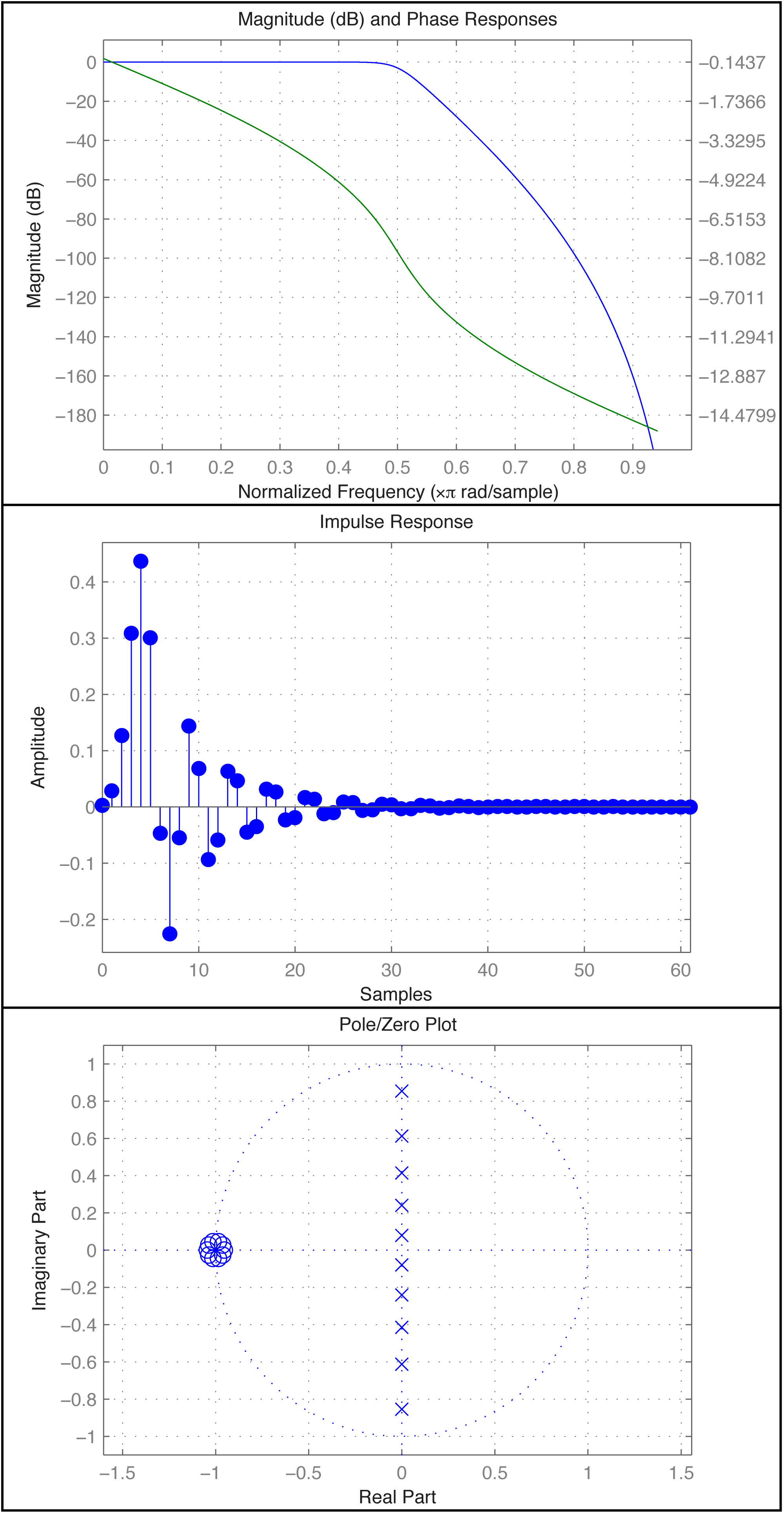
You can analyze the filter with the fvtool.

fvtool(a,b)

 

The fvtool provides a GUI through which you can see multiple views of the filter, including those in Figure 7.44. In the first figure, the blue line is the magnitude frequency response and the green line is phase.

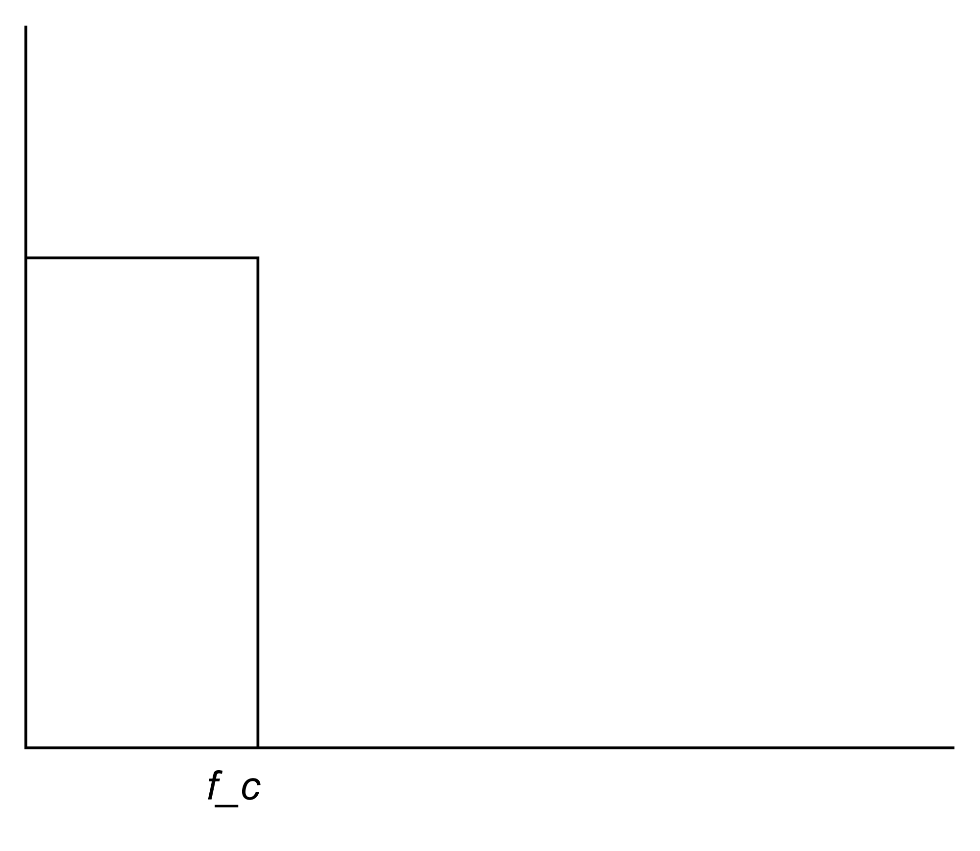
Another way to create and apply an IIR filter in MATLAB is by means of the function yulewalk. Let’s try a low-pass filter as a simple example. Figure 7.45 shows the idealized frequency response of a low-pass filter. The x-axis represents normalized frequencies, and f_c is the cutoff frequency. This particular filter allows frequencies that are up to ¼ the sampling rate to pass through, but filters out all the rest.

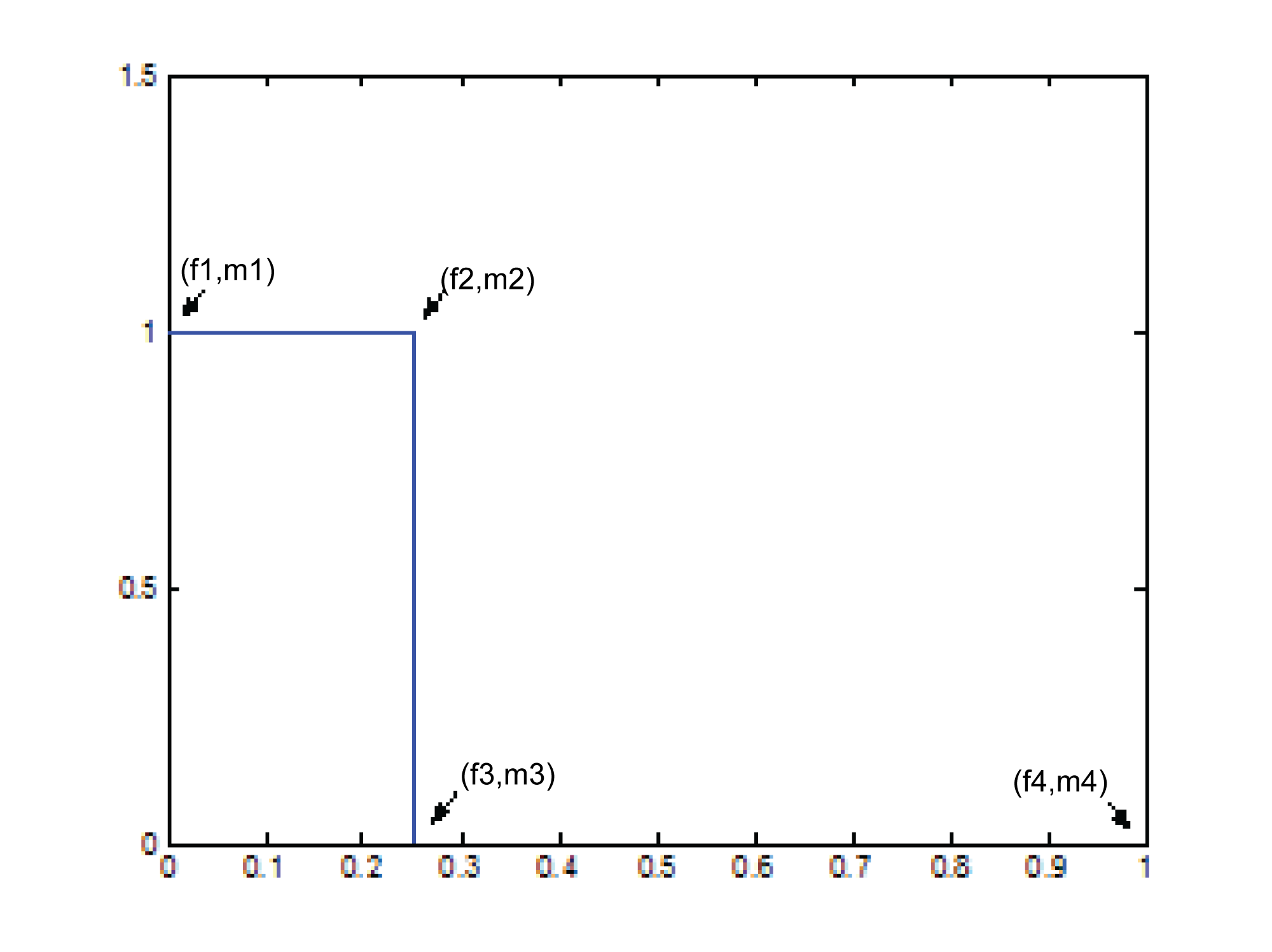
The first step in creating this filter is to store its “shape.” This information is stored in a pair of parallel vectors, which we’ll call f and m. For the four points on the graph in Figure 7.46, f stores the frequencies, and m stores the corresponding magnitudes. That is, $$\mathbf{f}=\left [ f1\; f2\; f3\; f4 \right ]$$ and $$\mathbf{m}=\left [ m1\; m2\; m3\; m4 \right ]$$, as illustrated in the figure. For the example filter we have

f = [0 0.25 0.25 1];

m = [1 1 0 0];

 

[aside]The yulewalk function in MATLAB is named for the Yule-Walker equations, a set of linear equations used in auto-regression modeling.[/aside]

Now that you have an ideal response, you use the yulewalk function in MATLAB to determine what coefficients to use to approximate the ideal response.

[a,b] = yulewalk(N,f,m)

 

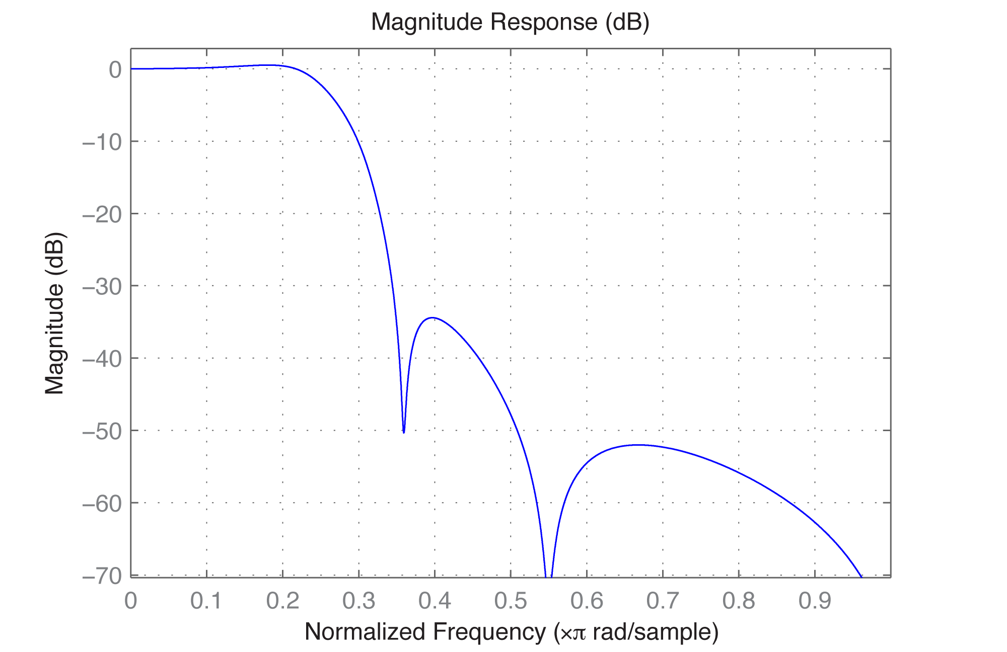
Again, an order N=6 filter is sufficient for the low-pass filter. You can use the same filter function as above to apply the filter. The resulting filter is given in Figure 7.47. Clearly, the filter cannot be perfectly created, as you can see from the large ripple after the cutoff point.

The finite counterpart to the yulewalk function is the fir2 function. Like butter, fir2 takes as input the order of the filter and two vectors corresponding to the shape of the filter’s frequency response. Thus, we can use the same f and m as before. fir2 returns the vector h constituting the filter.

h = fir2(N,f,m);

 

We need to use a higher order filter because this is an FIR. N=30 is probably high enough.

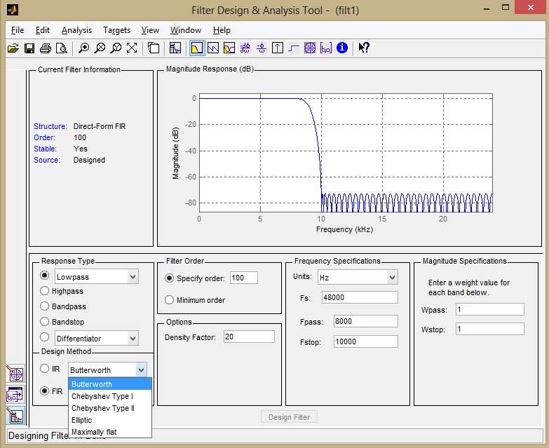
MATLAB’s extensive signal processing toolkit includes a Filter Designer with an easy-to-use graphical user interface that allows you to design the types of filters discussed in this chapter. A Butterworth filter is shown in Figure 7.48. You can adjust the parameters in the tool and see how the roll-off and ripples change accordingly. Experimenting with this tool helps you know what to expect from filters designed by different algorithms.

 

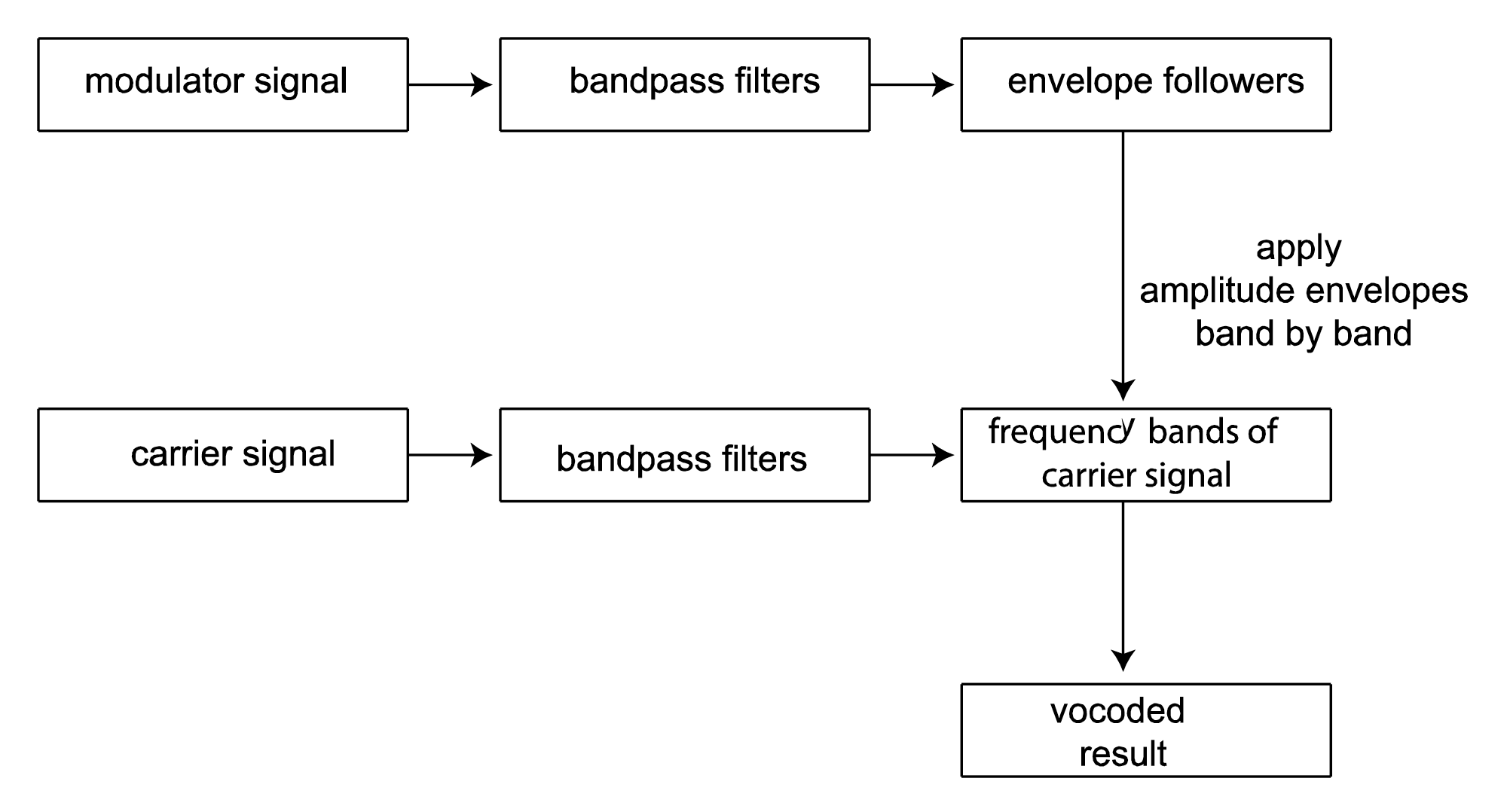
Vocoders were introduced in Section 7.1.8. The implementation of a vocoder is sketched in Algorithm 7.6 and diagrammed in Figure 7.49. The MATLAB and C++ exercises associated with this section encourage you to try your hand at the implementation.

[equation class=”algorithm” caption=”Algorithm 7.6 Sketch of an implementation of a vocoder”]

algorithm vocoder

/*

Input:

c, an array of audio samples constituting the carrier signal

m, n array of audio samples constituting the modulator signal

Output:

v, the carrier wave modulated with the modulator wave */

{

Initialize v with 0s

Divide the carrier into octave-separated frequency bands with bandpass filters

Divide the modulator into the same octave-separated frequency bands with bandpass filters for each band

use the modulator as an amplitude envelope for the carrier

}

[/equation]

[wpfilebase tag=file id=169 tpl=supplement /]

[wpfilebase tag=file id=103 tpl=supplement /]

[wpfilebase tag=file id=71 tpl=supplement /]

[wpfilebase tag=file id=101 tpl=supplement /]

Another interesting programming exercise is implementation of a pitch glide. A Risset pitch glide is an audio illusion that sounds like a constantly rising pitch. It is the aural equivalent of the visual image of a stripe on a barber pole that seems to be rising constantly. Implementing the pitch glide is suggested as an exercise for this section.

To this point, we’ve primarily considered off-line processing of audio data in the programs that we’ve asked you to write in the exercises.  This makes the concepts easier to grasp, but hides the very important issue of real-time processing, where operations have to keep pace with the rate at which sound is played.

Chapter 2 introduces the idea of audio streams.  In Chapter 2, we give a simple program that evaluates a sine function at the frequency of desire notes and writes the output directly to the audio device so that notes are played when the program runs.  Chapter 5 gives a program that reads a raw audio file and writes that to the audio device to play it as the program runs.  The program from Chapter 5 with a few modifications is given here for review.

/*Use option -lasound on compile line.  Send in number of samples and raw sound file name.*/

#include </usr/include/alsa/asoundlib.h>
#include <math.h>
#include <iostream>
using namespace std;

static char *device = "default";	/*default playback device */
snd_output_t *output = NULL;
#define PI 3.14159

int main(int argc, char *argv[])
{
        int err, numRead;
        snd_pcm_t *handle;
        snd_pcm_sframes_t frames;
        int numSamples = atoi(argv[1]);

        char* buffer = (char*) malloc((size_t) numSamples);
        FILE *inFile = fopen(argv[2], "rb");
        numRead = fread(buffer, 1, numSamples, inFile);
        fclose(inFile);   

        if ((err = snd_pcm_open(&handle, device, SND_PCM_STREAM_PLAYBACK, 0)) < 0){
            printf("Playback open error: %s\n", snd_strerror(err));
            exit(EXIT_FAILURE);
        }
        if ((err = snd_pcm_set_params(handle,
				SND_PCM_FORMAT_U8,
				SND_PCM_ACCESS_RW_INTERLEAVED,
				1,
				44100, 1, 400000) ) < 0 ){
            printf("Playback open error: %s\n", snd_strerror(err));
            exit(EXIT_FAILURE);
        }

        frames = snd_pcm_writei(handle, buffer, numSamples);
        if (frames < 0)
          frames = snd_pcm_recover(handle, frames, 0);
        if (frames < 0) {
          printf("snd_pcm_writei failed: %s\n", snd_strerror(err));
        }  
}

Program 7.1 Reading and writing raw audio data

This program uses the library function send_pcm_writei to send samples to the audio device to be played. The audio samples are read from in input file into a buffer and transmitted to the audio device without modification The variable buffer indicates where the samples are stored, and sizeof(buffer)/8 gives the number of samples given that this is 8-bit audio.

Consider what happens when you have a much larger stream of audio coming in and you want to process it in real time before writing it to the audio device. This entails continuously filling up and emptying the buffer at a rate that keeps up with the sampling rate.

Let’s do some analysis to determine how much time is available for processing based on a given buffer size. For a buffer size of N and a sampling rate of r, then $$N/r$$ seconds can be passed before additional audio data will be required for playing. For and $$N=4096$$ and $$r=44100$$, this would be $$\frac{4096}{44100}=0.0929\: ms$$. (This scheme implies that there will be latency between the input and output, at most $$N/r$$ seconds.)

What is you wanted to filter the input audio before sending it to the output? We’ve seen that filtering is more efficient in the frequency domain using the FFT. Assuming the input is in the time domain, our program has to do the following:

• convert data to the frequency domain with inverse FFT
• multiply the filter and the audio data
• convert data back to the time domain with inverse FFT
• write the data to the audio device

The computational complexity of the FFT and IFFT is $$0\left ( N\log N \right )$$, on the order of $$4096\ast 12=49152$$ operations (times 2). Multiplying the filter and the audio data is $$0\left ( N \right )$$, and writing the data to the audio devices is also $$0\left ( N \right )$$, adding on the order of the order of 2*4096 operations. This yields on the order of 106496 operations to be done in $$0.0929\; ms$$, or about $$0.9\; \mu s$$ per operation. Considering that today’s computers can do more than 100,000 MIPS (millions of instructions per second), this is not unreasonable.

We refer the reader to Boulanger and Lazzarini’s Audio Programming Book for more examples of real-time audio processing.

This book is intended to be useful to sound designers and technicians in theatre, film, and music production.  It is also aimed at computer scientists who would like to collaborate with such artists and practitioners or design the next generation of sound hardware and software for them.

We’ve provided a lot of information in previous chapters moving through the concepts, applications, and underlying science of audio processing.  In the end, we realize that most of our readers want to do something creative, whether designing and setting up the sound backdrop for a theatre performance, creating a soundtrack for film, producing music, or writing programs for innovative sound processing.  It’s doubtful and not even necessary that you mastered all the material in the previous chapters, but it serves as a foundation and a reference for your practical and artistic work.  In this chapter, we pull things together by going into more detail on the artists’ and practitioners’ hands-on work.

There are three main stages in the workflow for sound and music creation:  pre-production, when you design your project and choose your basic equipment; production, when you record and edit the sound; and post-production, when you mix and master the sound (for CDs and DVDs) and deliver it, either live or on a permanent storage medium.  In this chapter, we examine these three steps as they apply to sound, regardless of its ultimate purpose – including music destined for CD, DVD, or the web; sound scores for film or video; or music and sound effects for live theatre performances.  The three main stages can be further divided into a number of steps, with some variations depending on the purpose and delivery method of the sound.

• Pre-production

o   Designing and composing sound and music

o   Analyzing recording needs (choosing microphones, hardware and software, recording environment, etc.), making a schedule, and preparing for recording

• Production

o   Recording, finding, and/or synthesizing sound and music

o   Creating sound effects

o   Synchronizing

• Post-production

o   Audio processing individual tracks and mixing tracks (applying EQ, dynamics processing, special effects, stereo separation, etc.)

o   Overdubbing

o   Mastering (for CD and DVD music production)

o   Finishing the synchronization of sound and visual elements (for production of sound scores for film or video)

o   Channeling output

Clearly, all of this work is based on the first important, creative step – sound design and/or music composition.  Design and composition are very big topics in and of themselves and are beyond the scope of this book.  In what follows, we assume that for the most part the sound that is to be created has been designed or the music to be recorded has been composed, and you’re ready to make the designs and compositions come alive.

8.1.1.1 Making a Schedule

A logical place to begin as you initiative a project is by making a schedule for the creation of the different audio artifacts that make up the entire system.  Your project could be comprised of many different types of sounds, including live recordings (often on different tracks at different moments), existing recordings, Foley sound effects, MIDI-synthesized music or sound, or algorithmically-generated music or sound.  Some sounds may need to be recorded in the presence of others that have already been created, and these interdependencies determine your scheduling.  For example, if you’re going to record singers against a MIDI-sequenced backing track, the backing track will have to be created ahead of time – at least enough of the backing track so that that the singers are able to sing on pitch and in time with the music.

You also need to consider where and how the artifacts will be made.  Recording sessions may need to be scheduled and musicians hired.  Also, you’ll need to get the proper equipment ready for on-location or outdoor recording sessions.

To some extent you can’t plan out the entire process ahead of time. The creative process is messy and somewhat unpredictable. But the last thing you want is to run into some technical roadblock when the creative juices start flowing. So plan ahead as best you can to make sure that you have all the necessary elements in the right place at the right time as you work through the project.

8.1.1.2 Setting up for Recording

In Chapter 1, we introduced a wide variety of audio hardware and software.  We’ll now give an overview of different recording situations you might encounter and the equipment appropriate for each.

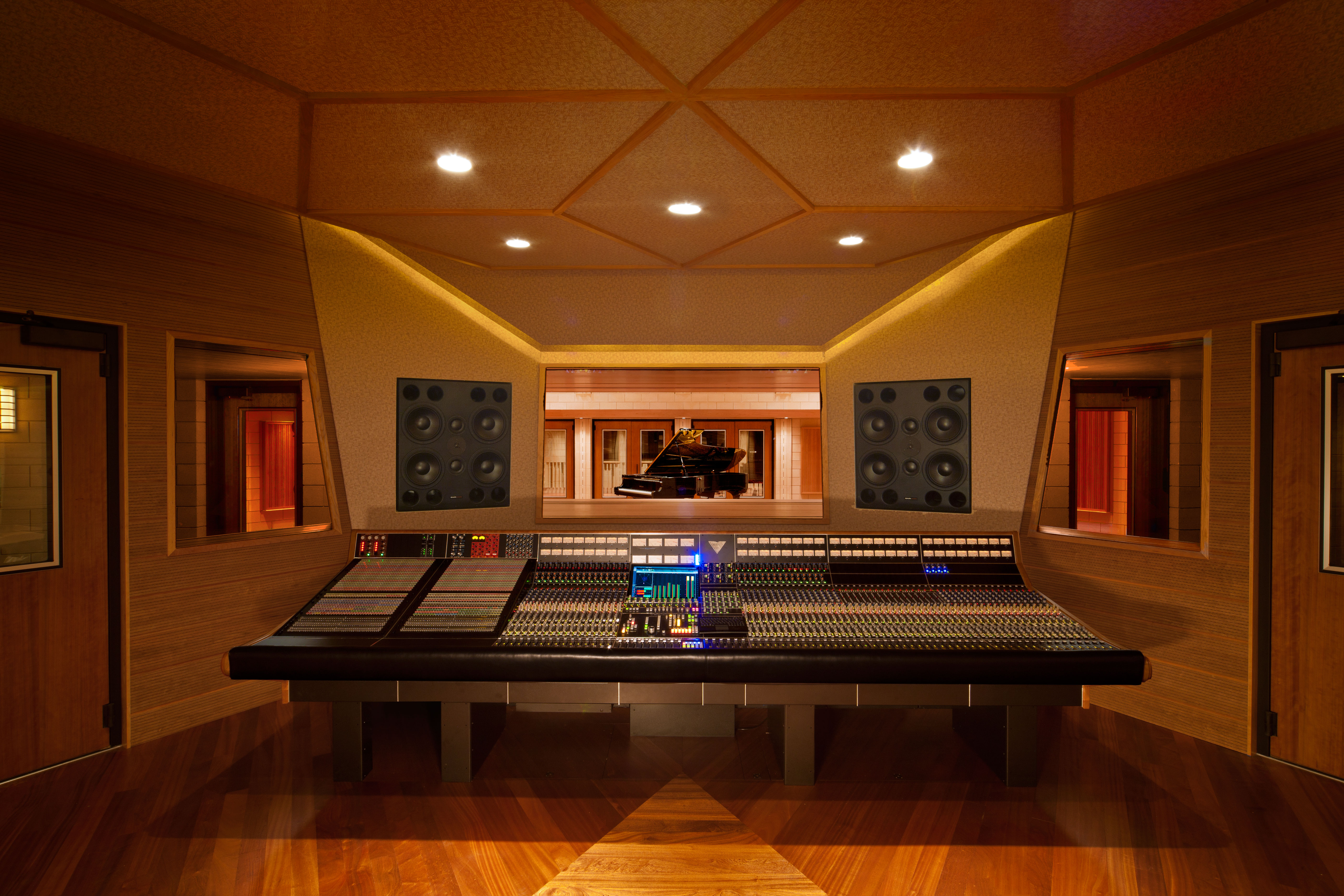
The ideal recording situation would be a professional recording studio. These studios typically have a large stage area where the performance can be recorded. Ideally, the stage has very meticulously controlled acoustics along with separate isolation booths, high-quality microphones, a control room that is isolated acoustically from the stage, and a professional recording engineer to conduct the recording. If you have enough money, you can rent time in these studios and get very good results. If you have a lot of money, you can build one yourself! Figure 8.1 shows an example of a world-class professional recording studio.

While you can get some really amazing recordings in a professional recording studio, you can still get respectable results by setting up your own recording environment using off-the-shelf tools. The first thing to do is find a place to record. This needs to be a quiet room without a lot of noise from the air handling and a fairly neutral acoustic environment. In other words, you usually don’t want to hear the room in your recordings. Examples of isolation rooms and techniques can be found in Chapter 4.

Once you have a room in which to make your recording you need a way to get some cables run into the room for your microphones as well as any headphones or other monitors required for the performer. These cables ultimately run back to wherever you are setting up your computer and recording interface. One thing to keep in mind is that, depending on how well your recording room is isolated from your control room, you may need to have a talkback microphone at your computer routed to the performer’s headphones. Some mixing consoles include a talkback microphone. A simple way to set up your own is to just connect a microphone to your audio interface and set up an extra recording track in your recording software. If that track is record-enabled, the performer will hear it along with his or her own microphone . You can also get a dedicated monitor management device that includes a talkback microphone and the ability to control and route the recording signal to all the various headphones and monitors for both you and the performer. An example of a monitor management device is shown in Figure 8.2.

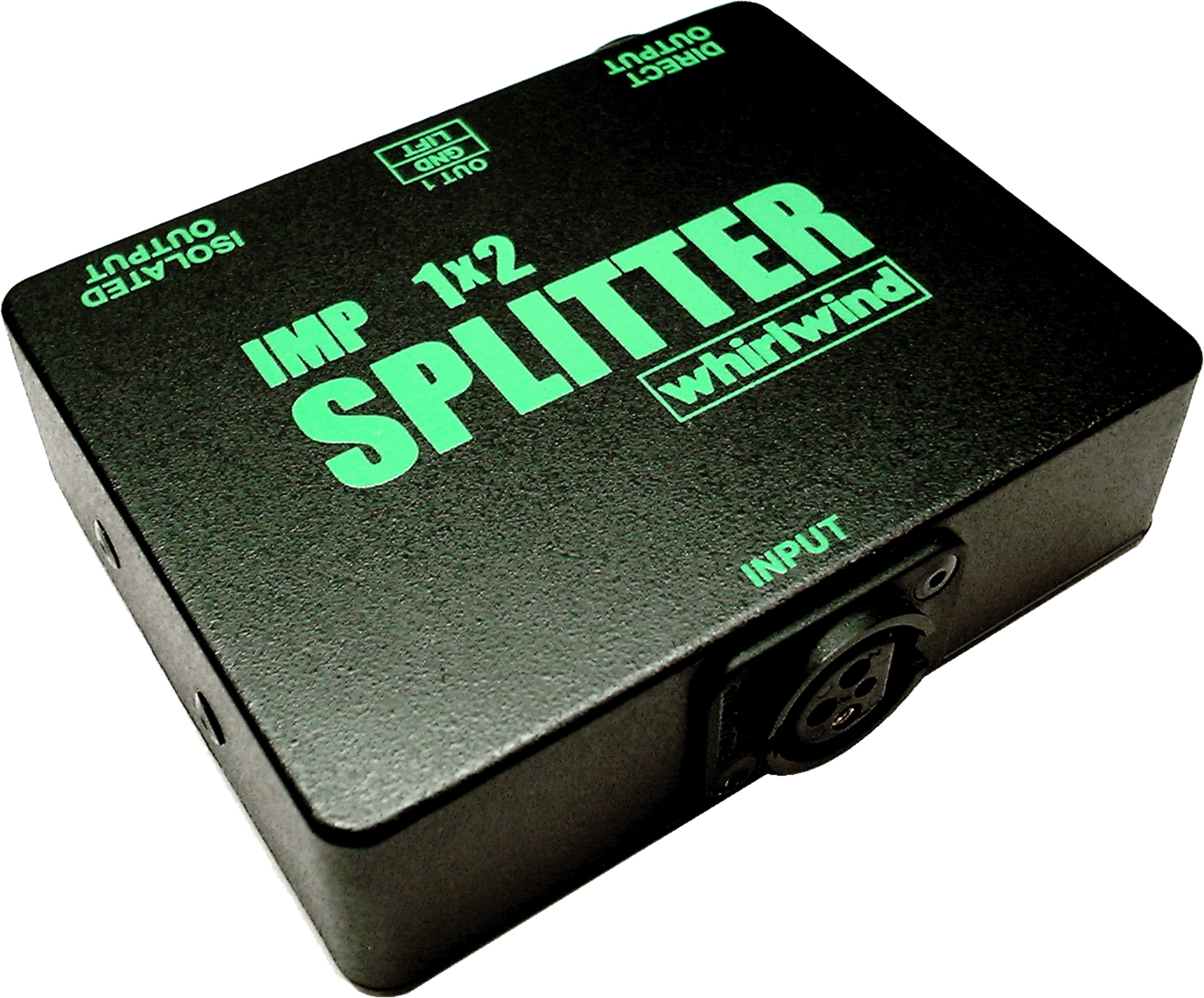
While it’s not technically a recording studio, you might find yourself in the situation where you need to record a live performance happening in a theatre, concert hall, or other live venue. The trick here is to get your recording without impacting the live performance. The simplest solution is to set up a couple area microphones on the stage somewhere and run them back to your recording equipment. If there are already microphones in place for live sound reinforcement, you can sometimes use those to get your recording. One way to do that is to work with the live sound engineer to get you a mix of all the microphones using an auxiliary output of the live mixing console. Assuming extra aux outputs are available, this is typically a simple thing to implement. Just make sure you speak with the engineer ahead of time about it. You won’t make any friends if you show up 15 minutes before the show starts and ask the engineer for a feed from the mixing console. The disadvantage to this is that you’re pretty much stuck with the mix that the live engineer gives you. Everything is already mixed. If you ask nicely you might be able to get two aux feeds with vocals on one and musical instruments on the other. This gives you a little more flexibility, but you are still limited to the mix that is happening on each aux feed. A better solution that requires more planning is to split the microphone signals to go to your recording equipment as well as the live mixing console. It is important to use a transformer-isolated splitter so it doesn’t negatively impact the live sound. These isolated splitters will essentially make your feed invisible to the live mixing console. You can get splitters with multiple channels or just single channel splitters like the one shown in Figure 8.3. With this strategy you can get a separate track for each microphone on the stage allowing you to create your own mix later when the live performance is over.

Sometimes you need to record something that is not practical to bring into a controlled environment like a recording studio. For example, if you want to record the sound of an airplane taking off, you’re going to have to go stand next to a runway at the airport with a microphone. This is called recording on-location. In these situations, the goal is to find a balance between fidelity, isolation, cost, and convenience. It’s very difficult to get all four of these things in every scenario, so compromises have to be made. The solution that offers the best isolation is not likely to be convenient and may be fairly expensive. For example, if you want to record thunder without picking up the sounds of rain, dog barks, cars, birds, and other environmental sounds, you need to find an outdoor location that is far from roads, houses, and trees but that also offers shelter from the rain for your equipment. Once you find that place, you need to predict when a thunderstorm will happen and get there in time to set up your equipment before the storm begins. Since this is not a very practical plan, you may have to make some compromises and be prepared to spend a long time recording storms in order to get a few moments where you manage to get the sound of thunder when nothing else is happening.  Every recording situation is different, but if you understand the options that are available, you can be better prepared to make a good decision.

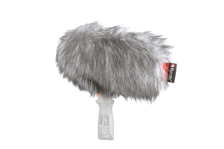
There are some unique equipment considerations you need to keep in mind when recording on-location. You may not have access to electricity so all your equipment may need to be battery-powered. We described some handheld, battery-powered recording devices in Chapter 1. Another common problem when recording on-location is wind. Wind blowing across a microphone will destroy your recording. Even a light breeze can be problematic. Most microphones come with a simple windscreen that can go over the microphone but in particularly windy conditions, a more robust windscreen may be necessary such as the one shown in Figure 8.4.

8.2.2.1 Capturing the Four-Dimensional Sound Field

When listening to sound in an acoustic space, such as at a live orchestral concert, you hear different sounds arriving from many directions. The various instruments are spread out on a stage, and their sound arrives at your ears somewhat spread out in time and direction according to the physical location of the instruments. You also hear subtly nuanced copies of the instrument sounds as they’re reflected from the room surfaces at even more varying times and directions. The audience makes their own sound in applause, conversation, shuffling in seats, cell phones going off, etc. These sounds arrive from different directions as well. Our ability to perceive this four-dimensional effect is the result of the physical characteristics of our hearing system. With two ears, the differences in arrival time and intensity between them allow us to perceive sounds coming from many different directions. Capturing this effect with audio equipment and then either reinforcing the live audio or recreating the effect upon playback is quite challenging.

The biggest obstacle is the microphone. A traditional microphone records the sound pressure amplitude at a single point in space. All the various sound waves arriving from different directions at different times are merged into a single electrical voltage wave on a wire. With all the data merged into a single audio signal, much of the four-dimensional acoustic information is lost. When you play that recorded sound out of a loudspeaker, all the reproduced sounds are now coming from a single direction as well. Adding more loudspeakers doesn’t solve the problem because then you just have every sound repeated identically from every direction, and the precedence effect will simply kick in and tell our brain that the sound is only coming from the lone source that hits our ears first.

[aside]If the instruments are all acoustically isolated, the musicians may have a hard time hearing themselves and each other. This poses a significant obstacle, as they will have a difficult time trying to play together. To address this problem, you have to set up a complicated monitoring system.  Typically each musician has a set of headphones that feeds him or her a custom mix of the sounds from each mic/instrument.[/aside]

The first step in addressing some of these problems is to start using more than one microphone. Stereo is the most common recording and playback technique. Stereo is an entirely man-made effect, but produces a more dynamic effect upon playback of the recorded material with only one additional loudspeaker. The basic idea is that since we have two ears, two loudspeakers should be sufficient to reproduce some of the four-dimensional effects of acoustic sound. It’s important to understand that there is no such thing as stereo sound in an acoustic space. You can’t make a stereo recording of a natural sound. When recording sound that will be played back in stereo, the most common strategy is recording each sound source with a dedicated microphone that is as acoustically isolated as possible from the other sound sources and microphones. For example, if you were trying to record a simple rock band, you would put a microphone on each drum in the drum kit as close to the drum as possible. For the electric bass, you would put a microphone as close as possible to the amplifier and probably use a hardwired cable from the instrument itself. This gives you two signals to work with for that instrument. You would do the same for the guitar. If possible, you might even isolate the bass amplifier and the guitar amplifier inside acoustically sealed boxes or rooms to keep their sound from bleeding into the other microphones. The singer would also be isolated in a separate room with a dedicated microphone.

During the recording process, the signal from each microphone is recorded on a separate track in the DAW software and written to a separate audio file on the hard drive. With an isolated recording of each instrument, a mix can be created that distributes the sound of each instrument between two channels of audio that are routed to the left and right stereo loudspeaker. To the listener sitting between the two loudspeakers, a sound that is found only on the left channel sounds like it comes from the left of the listener and vice versa for the right channel. A sound mixed equally into both channels appears to the listener as though the sound is coming from an invisible loudspeaker directly in the middle. This is called the phantom center channel. By adjusting the balance between the two channels, you can place sounds at various locations in the phantom image between the two loudspeakers. This flexibility in mixing is possible only because each instrument was recorded in isolation. This stereo mixing effect is very popular and produces acceptable results for most listeners.

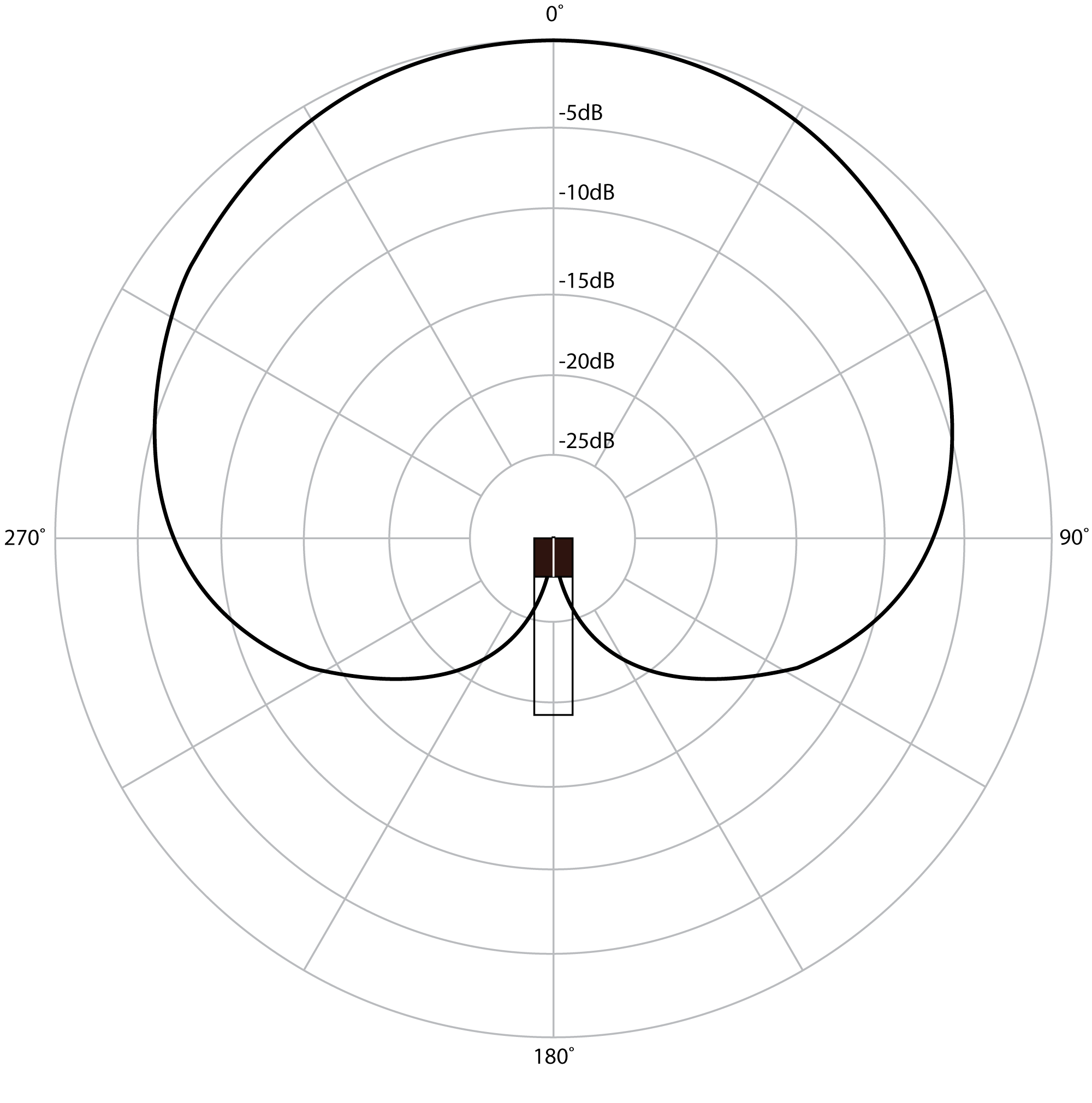
When recording in a situation where it’s not practical to use multiple microphones in isolation – such as for a live performance or a location recording where you’re capturing an environmental sound – it’s still possible to capture the sound in a way that creates a stereo-like effect. This is typically done using two microphones and manipulating the way the pickup patterns of the microphones overlap. Figure 8.5 shows a polar plot for a cardioid microphone. Recall that a cardioid microphone is a directional microphone that picks up the sound very well on-axis with the front of the microphone but doesn’t pick up the sound as well off-axis. This polar plot shows only one plotted line, representing the pickup pattern for a specific frequency (usually 1 kHz), but keep in mind that the directivity of the microphone changes slightly for different frequencies. Lower frequencies are less directional and higher frequencies are more directional than what is shown in Figure 8.5. With that in mind, we can examine the plot for this frequency to get an idea of how the microphone responds to sounds from varying directions. Our reference level is taken at 0° (directly on-axis). The dark black line representing the relative pickup level of the microphone intersects with the 0 dB line at 0°. As you move off-axis, the sensitivity of the microphone changes. At around 75°, the line intersects with the -5 dB point on the graph, meaning that at that angle, the microphone picks up the sound 5 dB quieter than it does on-axis. As you move to around 120°, the microphone now picks up the sound 15 dB quieter than the on-axis level. At 180° the level is null.

One strategy for recording sound with a stereo effect is to use an XY cross pair. The technique works by taking two matched cardioid microphones and positioning them so the microphone capsules line up horizontally at 45° angles that cross over the on-axis point of the opposite microphone. Getting the capsules to line up horizontally is very important because you want the sound from every direction to arrive at both microphones at the same time and therefore in the same phase.

[aside]At 0° on-axis to the XY pair, the individual microphone elements are still tilted 45°, making the microphone’s pickup a few dB quieter than its own on-axis level would be.  Yet because the sound arrives at both microphones at the same level and the same phase, the sound is perfectly reinforced, causing a boost in amplitude.  In this case the result is actually slightly louder than the on-axis level of either individual microphone.[/aside]

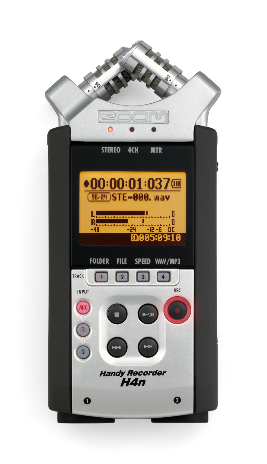
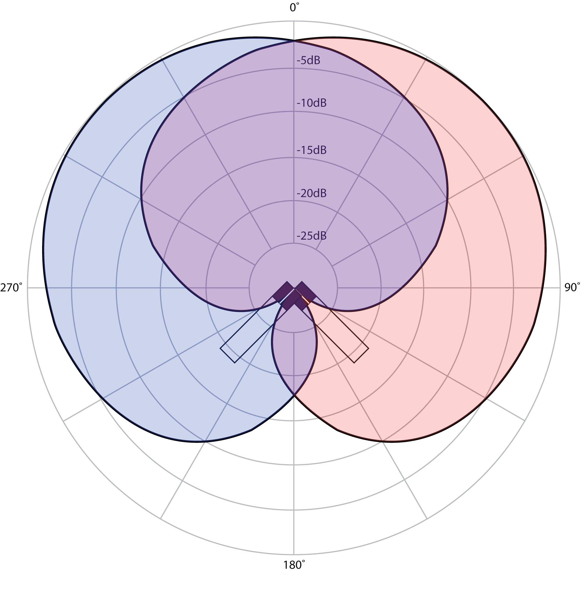
Figure 8.6 shows a recording device with integrated XY cross pair microphones, and Figure 8.7 shows the polar patterns of both microphones when used in this configuration. The signals of these two microphones are recorded onto separate tracks and then routed to separate loudspeakers for playback. The stereo effect happens when these two signals combine in the air from the loudspeakers. Let’s first examine the audio signals that are unique to the left and right channels. For a sound that arrives at the microphones 90° off-axis, there is approximately a 15 dB difference in level for that sound captured between the two microphones. As a rule of thumb, whenever you have a level difference that is 10 dB or greater between two similar sounds, the louder sound takes precedence. Consequently, when that sound is played back through the two loudspeakers, it is perceived as though it’s entirely located at the right loudspeaker. Likewise, a sound arriving 270° off-axis sounds as though it’s located entirely at the left loudspeaker. At 0°, the sound arrives at both microphones at the same level. Because the sound is at an equal level in both microphones, and therefore is played back equally loud through both loudspeakers, it sounds to the listener as if it’s coming from the phantom center image of the stereo field. At 45°, the polar plots tell us that the sound arrives at the right microphone approximately 7 dB louder than at the left. Since this is within the 10 dB range for perception, the level in the left channel causes the stereo image of the sound to be pulled slightly over from the right channel, now seeming to come from somewhere between the right speaker and the phantom center location. If the microphones are placed appropriately relative to the sound being recorded, this technique can provide a fairly effective stereo image without requiring any additional mixing or panning.

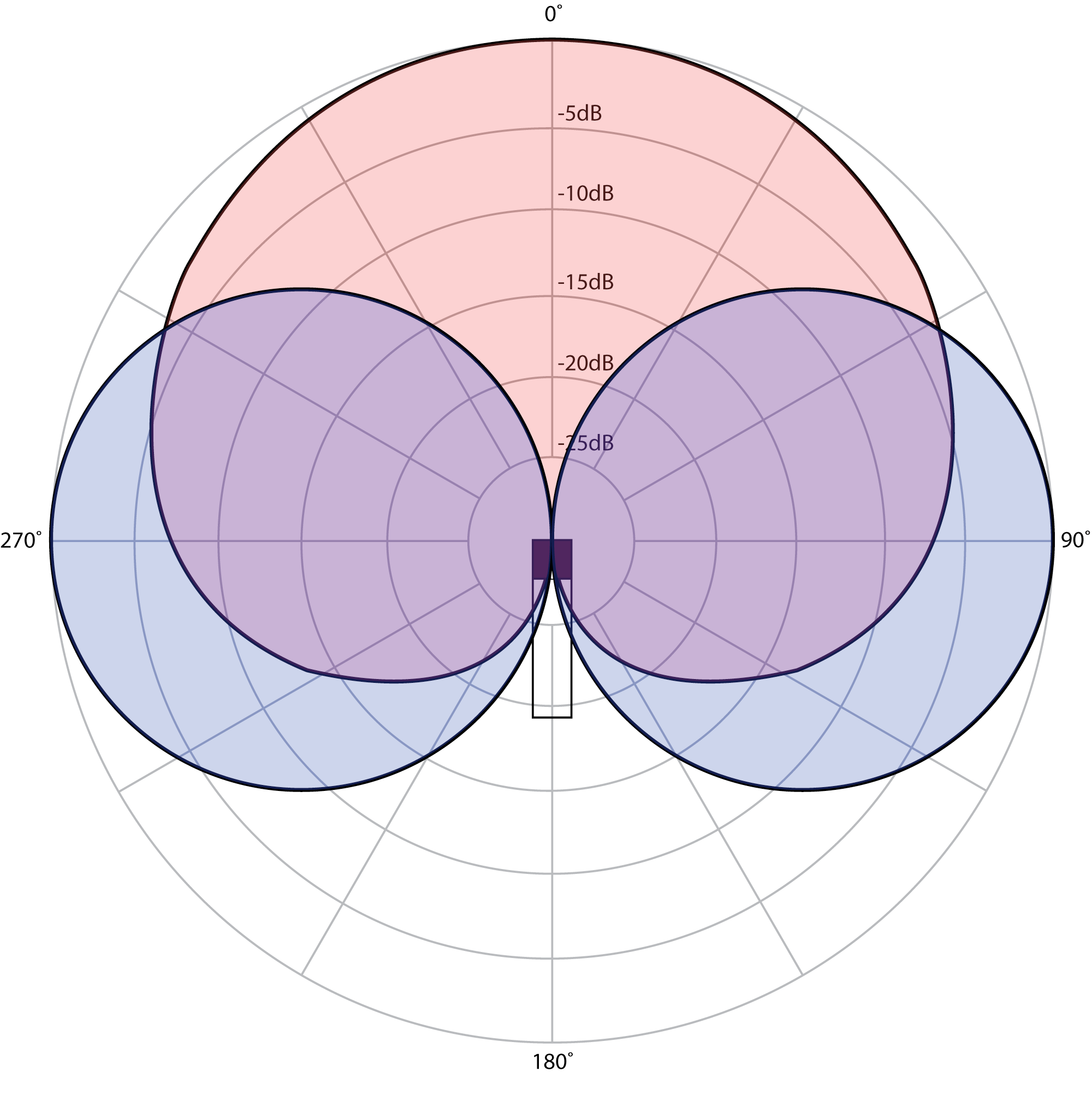
Another technique for recording a live sound for a stereo effect is called mid-side. Mid-side also uses two microphones, but unlike XY, one microphone is a cardioid microphone and the other is a bidirectional or figure-eight microphone. The cardioid microphone is called the mid microphone and is pointed forward (on-axis), and the figure-eight microphone is called the side microphone and is pointed perpendicular to the mid microphone. Figure 8.8 shows the polar patterns of these two microphones in a mid-side configuration.

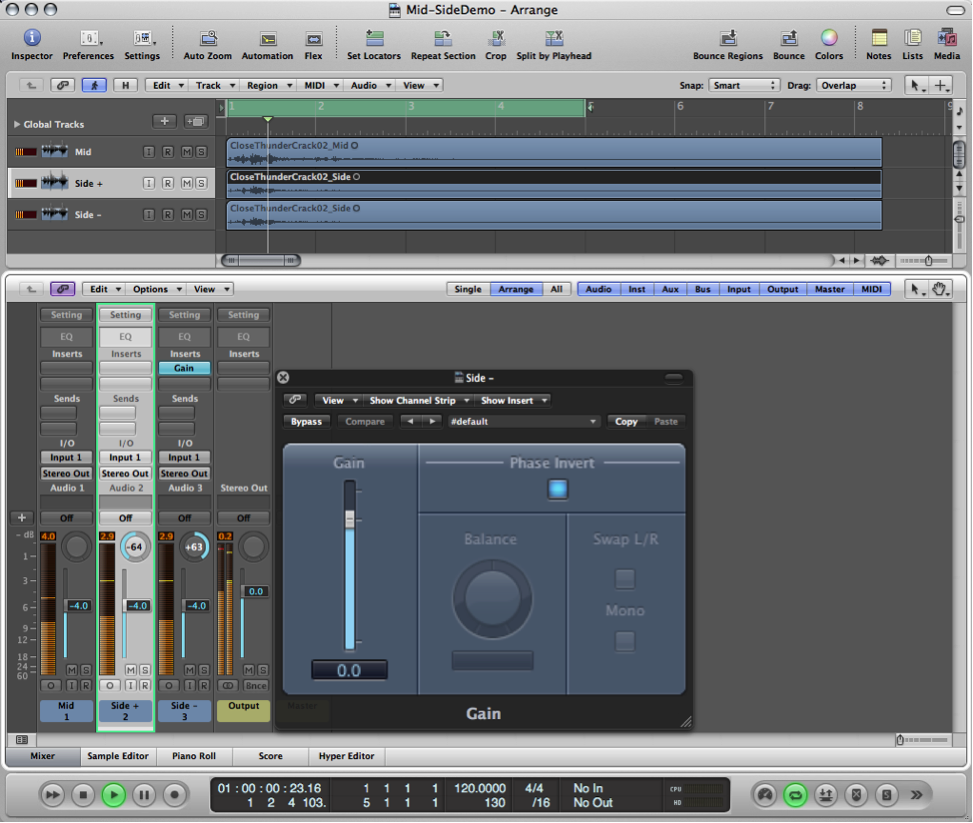
The side microphone has a single diaphragm that responds to pressure changes on either side of the microphone. The important thing to understand here is that because of the single diaphragm, the sounds on either side of the microphone are captured in opposite polarity.  That is, a sound that causes a positive impulse on the right of the microphone causes a negative impulse on the left of the microphone. It is this polarity effect of the figure-eight microphone that allows the mid-side technique to work. After you’ve recorded the signal from these two microphones onto separate channels, you have to set up a mid-side matrix decoder in your mixing console or DAW software in order to create the stereo mix. To create a mid-side matrix, you take the audio from the mid microphone and route it to both left and right output channels (pan center). The audio from the side microphone gets split two ways. First it gets sent to the left channel (pan left).  Then it gets sent also to the right channel (pan right) with the polarity inverted.  Figure 8.9 shows a mid-side matrix setup in Logic. The “Gain” plugin inserted on the “Side -” track is being used only to invert the polarity (erroneously labeled “Phase Invert” in the plug-in interface).

Through the constructive and destructive combinations of the mid and side signals at varying angles, this matrix creates a stereo effect at its output. The center image is essentially derived from the on-axis response of the mid microphone, which by design happens also to be the off-axis point of the side microphone.  Any sound that arrives at 0° to the mid microphone is added to both the left and right channels without any interaction from the signal from the side microphone, since at 0° to the mid-side setup the side microphone pickup is null. If you look at the polar plot, you can see that the mid microphone picks up every sound within a 120° spread with only 6 dB or so of variation in level.  Aside from this slight level difference, the mid microphone doesn’t contain any information that can alone be used to determine a sound’s placement in the stereo field.  However, approaching the 300° point (arriving more from the left of the mid-side setup), you can see that the sound arriving at the mid microphone is also picked up by the side microphone at the same level and the same polarity. Similarly, a sound that arrives at 60° also arrives at the side microphone at the same level as the mid, but this time it is inverted in polarity from the signal at the mid microphone.  If you look at how these two signals combine, you can see that the mid sound at 300° mixes together with the “Side +” track and, because it is the same polarity, it reinforces in level. That same sound mixes together with the “Side -” track and cancels out because of the polarity inversion.  The sound that arrives from the left of the mid-side setup therefore is louder on the left channel and accordingly appears to come from the left side of the stereo field upon playback.  Conversely, a sound coming from the right side at 60° reinforces when mixed with the “Side-“ track but cancels out when mixed with the “Side+” track, and the matrixed result is louder in the right channel and accordingly appears to come from the right of the stereo field.  Sounds that arrive between 0° and 300° or 0° and 60°have a more moderate reinforcing and canceling effect, and the resulting sound appears at some varying degree between left, right, and center depending on the specific angle. This creates the perception of sound that is spread between the two channels in the stereo image.

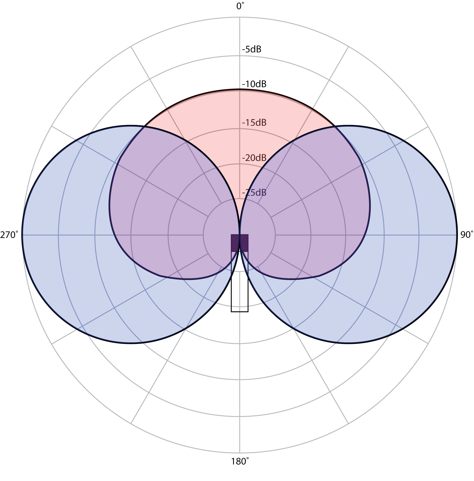
The result here is quite similar to the XY cross pair technique with one significant difference. Adjusting the relative level of the “Mid” track alters the spread of the stereo image. Figure 8.10 shows a mid-side polar pattern with the mid microphone attenuated -10 dB. Notice that the angle where the two microphones pick up the sound at equal levels has narrowed to 45° and 315°. This means that when they are mixed together in the mid-side matrix, a smaller range of sounds are mixed equally into both left and right channels. This effectively widens the stereo image. Conversely, increasing the level of the mid microphone relative to the side microphone causes more sounds to be mixed into the left and right channels equally, thereby narrowing the stereo image. Unlike the XY cross pair, with mid-side the stereo image can be easily manipulated after the recording has already been made.

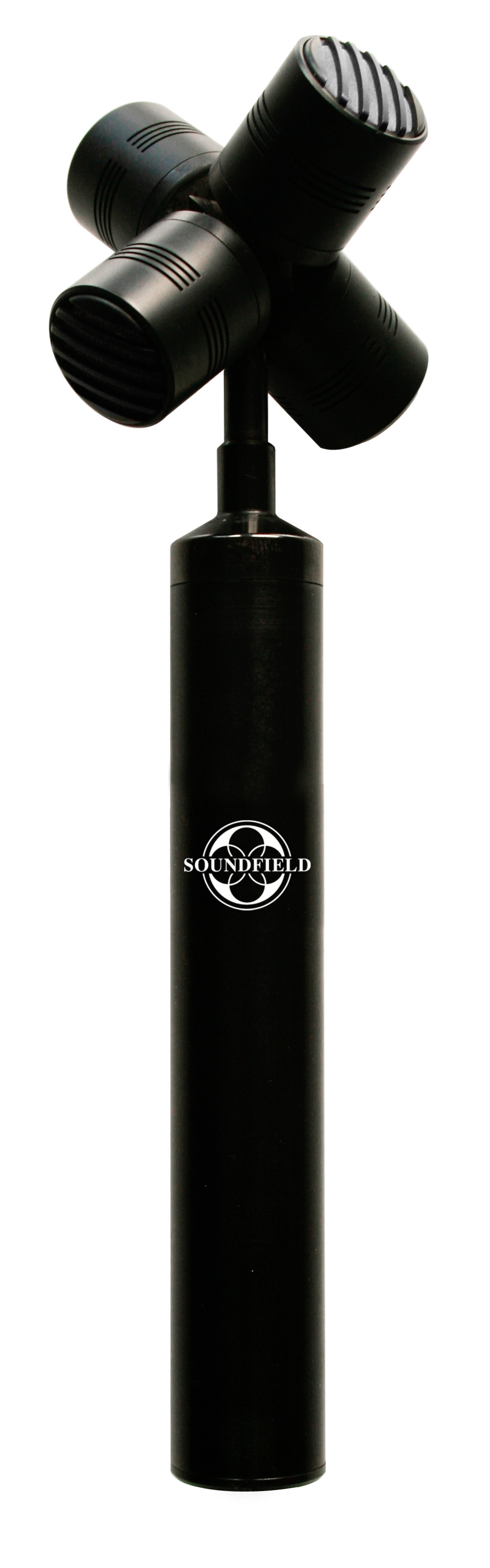
The concept behind mid-side recording can be expanded in a number of ways to allow recordings to capture sound in many directions while still maintaining the ability to recreate the desired directional information on playback. One example is shown in Figure 8.11.  This microphone from the Soundfield Company has four microphone capsules in a tetrahedral arrangement, each pointing a different direction. Using proprietary matrix processing, the four audio signals captured from this microphone can be combined to generate a mono, stereo, mid-side, four-channel surround, five-channel surround, or even a seven-channel surround signal.

The counterpart to setting up microphones for stereo recording is setting up loudspeakers for stereo listening.  Thus, we touch on the mid-side technique in the context of loudspeakers in Section 8.2.4.5.

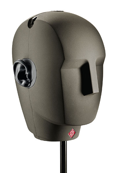
The most simplistic (and arguably the most effective) method for capturing four-dimensional sound is binaural recording. It’s quite phenomenal that despite having only two transducers in our hearing system (our ears), we are somehow able to hear and perceive sounds from all directions. So instead of using complicated setups with multiple microphones, just by putting two microphones inside the ears of a real human, you can capture exactly what the two ears are hearing.  This method of capture inherently includes all of the complex inter-aural time and intensity difference information caused by the physical location of the ears and the human head that allows the brain to decode and perceive the direction of the sound. If this recorded sound is then played back through headphones, the listener perceives the sound almost exactly as it was perceived by the listener in the original recording. While wearable headphone-style binaural microphone setups exist, sticking small microphones inside the ears of a real human is not always practical, and an acceptable compromise is to use a binaural dummy head microphone. A dummy head microphone is essentially the plastic head of a mannequin with molds of a real human ear on either side of the head. Inside each of these prosthetic ears is a small microphone, the two together capturing a binaural recording. Figure 8.12 shows a commercially available dummy head microphone from Neumann.

With binaural recording, the results are quite effective. All the level, phase, and frequency response information of the sound arriving at both ears individually that allows us to perceive sound is maintained in the recording. The real limitation here is that the effect is largely lost when the sound is played through loudspeakers. The inter-aural isolation provided by headphones is required when listening to binaural recordings in order to get the full effect.

[wpfilebase tag=file id=125 tpl=supplement /]

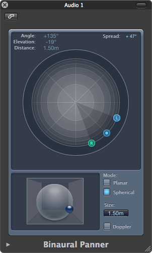
A few algorithms have been developed that mimic the binaural localization effect. These algorithms have been implemented into binaural panning plug-ins that are available for use in many DAW software programs, allowing you to artificially create binaural effects without requiring the dummy head recordings. An example of a binaural panning plug-in is shown in Figure 8.13. One algorithm is called the Cetera algorithm and is owned by the Starkey hearing aid company. They use the algorithm in their hearing aids to help the reinforced sound from a hearing aid sound more like the natural response of the ear. Starkey created a demo of their algorithm called the Starkey Virtual Barbershop. Although this recording sounds like it was captured with a binaural recording system, the binaural localization effects are actually rendered on a computer using the Cetera algorithm.

8.2.2.2 Setting Levels for Recording

Before you actually hit the “record” button you’ll want to verify that all your input levels are correct. The goal is to adjust the microphone preamplifiers so the signal from each microphone is coming into the digital converters at the highest voltage possible without clipping. Start by record-enabling the track in your software and then have the performer do the loudest part of his or her performance. Adjust the preamplifier so that this level is at least 6 dB below clipping. This way when the performer sings or speaks louder, you can avoid a clip. While recording, keep an eye on the input meters for each track and make sure nothing clips. If you do get a clip, at the very least you need to reduce the input gain on the preamplifier. You may also need to redo that part of the recording if the clip was bad enough to cause audible distortion.

8.2.2.3 Multitrack Recording

As you learned in previous chapters, today’s recording studios are equipped with powerful multitrack recording software that allows you to record different voices and instruments on different tracks. This environment requires that you make choices about what elements should be recorded at the same. For example, if you’re recording music using real instruments, you need to decide whether to record everything at the same time or record each instrument separately. The advantage to recording everything at the same time is that the musicians can play together and feel their way through the song. Musicians usually prefer this, and you almost always get a better performance when they play together. The downside to this method is that with all the musicians playing in the same room, it’s difficult to get good isolation between the instruments in the recording. Unless you’re very careful, you’ll pick up the sound of the drums on the vocalist’s microphone. This is hard to fix in post-production, because if you want the vocals louder in the mix, the drums get louder, also.

If you decide to record each track separately, your biggest problem is going to be synchronization. If all the various voices and instruments are not playing together, they will not be very well synchronized. They will start and end their notes at slightly different times, they may not blend very well, and they may not all play at the same tempo. The first thing you need to do to combat this problem is to make sure the performer can hear the other tracks that have already been recorded. Usually this can be accomplished by giving the performer a set of headphones to wear that are connected to your audio interface. The first track you record will set the standard for tempo, duration, etc. If the subsequent tracks can be recorded while the performer listens to the previous ones, the original track can set the tempo. Depending on what you are recording, you may also be able to provide a metronome or click track for the performers to hear while they perform their track. Most recording software includes a metronome or click track feature. Even if you use good monitoring and have the performers follow a metronome, there will still be synchronization issues. You may need to have them do certain parts several times until you get one that times out correctly. You may also have to manipulate the timing after the fact in the editing process.

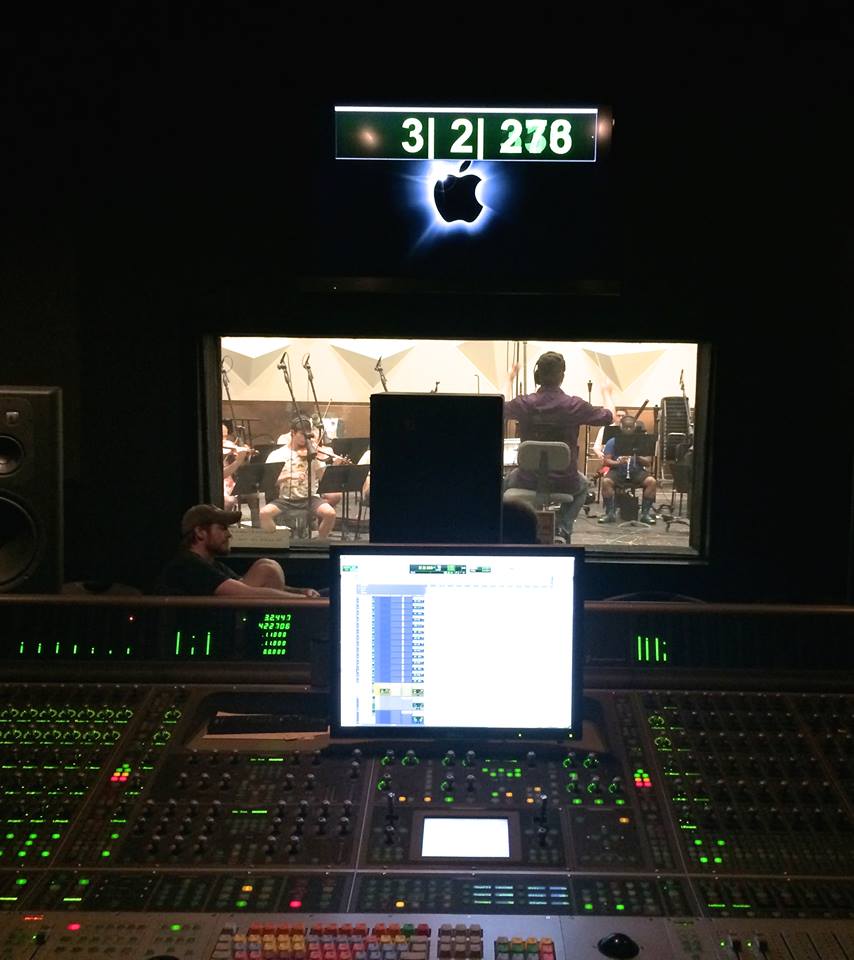
Figure 8.14 shows a view from the mixing console during a recording session for a film score. You can see through the window into the stage where the orchestra is playing. Notice that the conductor and other musicians are wearing headphones to allow them to hear each other and possibly even the metronome associated with the beat map indicated by the timing view on the overhead screen. These are all strategies for avoiding synchronization issues with large multi-track recordings.

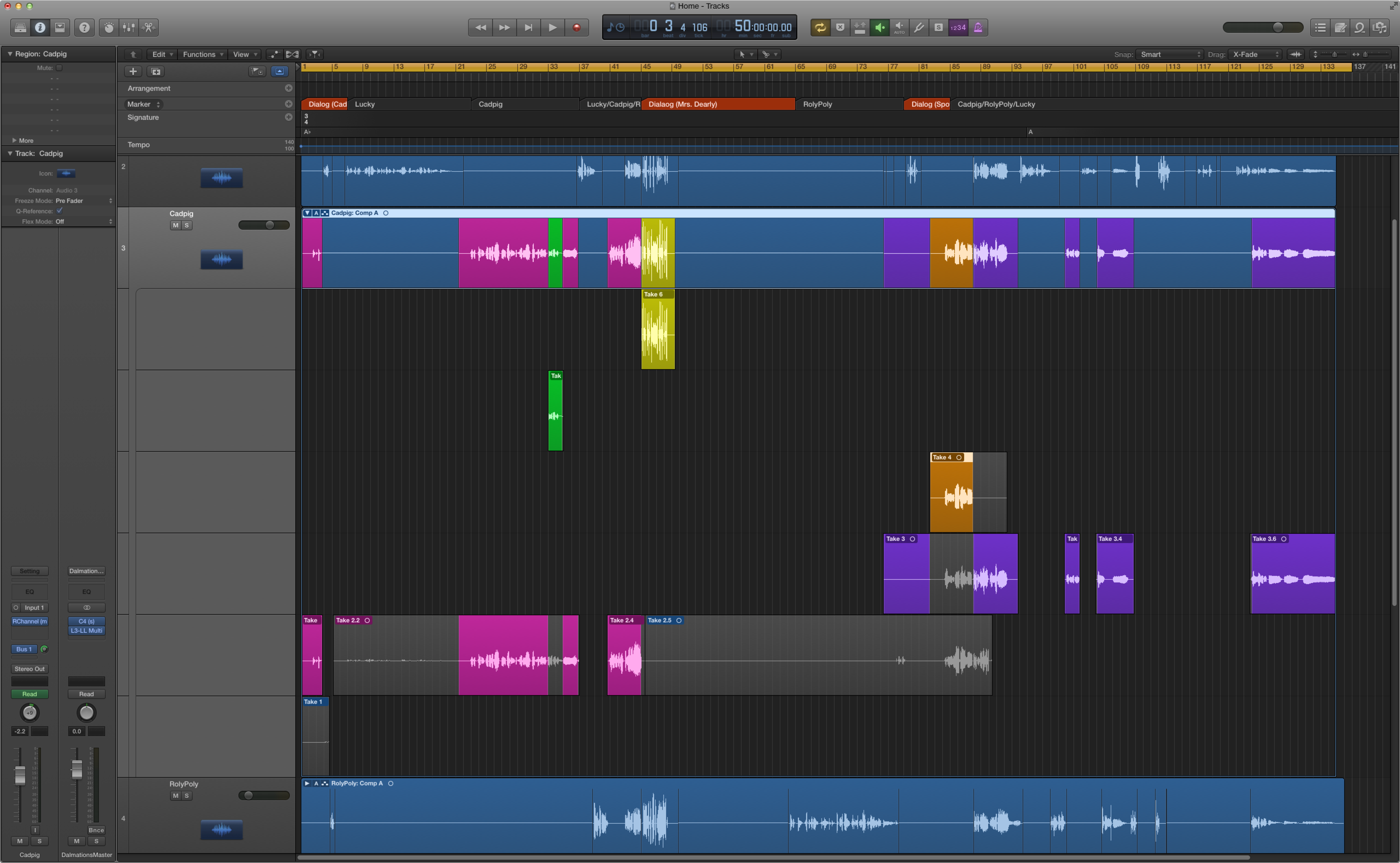
Another issue you will encounter in nearly every recording is that performers will make mistakes. Often the performer will need to make several attempts at a given performance before an acceptable performance is recorded. These multiple attempts are called takes, and each take represents a separate recording of the performer attempting the same performance. In some cases a given take may be mostly acceptable, but there was one small mistake. Instead of doing an entire new take, you can just re-record that short period of the performance that contained the mistake. This is called punch-in recording.

To make a punch-in recording you set up a start and stop time marker and start playback on the session. The performer hears the preceding several seconds and starts singing along with the recording. When the timeline encounters the start marker, the software starts writing the recording to the track and then reverts back to playback mode when the stop marker is reached. In the end you will have several takes and punch-ins folded into a single track. This is called a composite track, usually abbreviated to comp. A comp track allows you to unfold the track to see all the various takes. You can then go through them and select all the parts you want to keep from each take. A composite single version is created from all the takes you select. Figure 8.15 shows a multi-track recording session in Logic that uses a composite track that has been unfolded to show each take. The comp track is at the top and is color-coded to indicate which take was used for each period of time on the track.

8.2.2.4 Recording Sound for Film or Video

Production audio for film or video refers to the sound captured during the production process – when the film or video is actually being shot. In production, there may be various sounds you’re trying to capture – the voices of the actors, environmental sounds, sounds of props, or other scenic elements. When recording in a controlled sound stage studio, you generally can capture the production audio with reasonably good quality, but when recording on location you constantly have to battle background noise. The challenge in either situation is to capture the sounds you need without capturing the sounds you don’t need.

All the same rules apply in this situation as in other recording situations. You need good quality microphones, and you need to get them as close as possible to the thing you’re trying to record. Microphone placement can be challenging in a production environment where high definition cameras are close up on actors, capturing a lot of detail. Typically the microphone needs to be invisible or out of the camera shot. Actors can wear wireless lavaliere microphones as long as they can be hidden under some clothing. This placement affects the quality of the sound being picked up by the microphone, but in the production environment compromises are a necessity. The primary emphasis is of course on capturing the things that would be impossible or expensive to change in post-production, like performances or action sequences. For example, if you don’t get the perfect performance from the actors, or the scenery falls down, it’s very difficult to fix the problem without completely repeating the entire production process. On the other hand, if the production audio is not captured with a high enough quality, the actor can be brought back in alone to re-record the audio without having to reshoot the video. The bottom line is that in the production environment, the picture and the performance are the most important things. Capturing the production audio is ultimately of less importance because it’s easier to fix in post-production.

With this in mind, most production audio engineers are willing to make some compromises by putting microphones under the clothing. The other option is to mount a small directional microphone to a long pole called a boom pole. Someone outside the camera shot holds the pole, and he or she can get the microphone fairly close to actors or objects without getting the microphone in the shot. Because reshooting is so expensive, the most important job of the boom pole operator is to keep the microphone out of the shot. Picking up usable production audio is secondary.

Musical scores are another major element in film and video. Composers typically work first on developing a few musical themes to be used throughout the film while the editing process is still happening. Once a full edit is completed, the composer takes the themes and creates versions of various lengths to fit with the timing of the edited scenes. Sometimes this is done entirely with electronic instruments directly in the DAW with the video imported to the project file for a visual reference. Other times, a recording session is conducted where an orchestra is brought into a recording studio called a scoring stage. The film is projected in the studio and the composer along with a conductor performs the musical passages for the film using clicks and streamers to help synchronize the important moments.

A final challenge to be mentioned in the context of film and video is the synchronization of sound and picture. The audio is typically captured on a completely different recording medium than the video or film, and the two are put back together in post-production. In the analog domain this can be a very tricky process. The early attempt at facilitating synchronization was the clapboard slate. The slate has an area where you can write the name of the show, the scene number, and the take number. There is also a block of wood connected to the slate with a hinge. This block of wood can be raised and lowered quickly onto the slate to make a loud clap sound. The person holding the slate reads out loud the information written on the slate while holding the slate in front of the camera and then drops the clapper. In post-production the slate information can be seen on the film and heard on the audio recording. This way you know that you have the correct audio recording with the correct video. The clap sound can easily be heard on the audio recording, and on the video you can easily see the moment that the clapper closes. The editor can line up the sound of the clap with the image of the clapper closing, and then everything after that is in sync. This simple and low-tech solution has proven to be quite effective and is still used in modern filmmaking along with other improvements in synchronization technology.

A time code format called SMPTE has been developed to address the issue of synchronization. The format of SMPTE time code is described in Chapter 6. The idea behind time code synchronization is that the film has a built-in measuring system. There are 24 frames or still pictures every second in traditional motion picture film, with each frame being easily identified. The problem is that on an audiotape there is no inherent way to know which part of audio goes with which frame of video. Part of the SMPTE time code specification includes a method of encoding the time code into an audio signal that can be recorded on a separate track of audio on the tape recorder. This way, the entire audio recording is linked to each frame of the video. In the digital domain, this time code can be encoded into the video signal as well as the audio signal, and the computer can keep everything in sync. The slate clapper has even been updated to display the current time code value to facilitate synchronization in post-production.

8.2.2.5 Sound Effects

Sound effects are important components in film, video, and theatre productions. Sound effects are sometimes referred to as Foley sound, named after Jack Foley, who did the original work on sound effect techniques in the early days of silent films. Foley artists are a special breed of filmmaker who create all the sound effects for a film manually in a recording session. Foley stages are recording studios with all kinds of toys, floor surfaces, and other gadgets that make various sounds. The Foley artists go into the stage and watch the film while performing all the sounds required, the sounds ranging from footsteps and turning doorknobs to guns, rain, and other environmental sounds. The process is a lot of fun, and some people build entire careers as Foley artists.

[wpfilebase tag=file id=144 tpl=supplement /]

The first step in the creation of sound effects is acquiring some source material to work with. Commercial sound effect libraries are available for purchase, and there are some online sources for free sound effects, but the free sources are often of inconsistent quality. Sometimes you may need to go out and record your own source material. The goal here is not necessarily to find the exact sound you are looking for. Instead, you can try to find source material that has some of the characteristics of the sound. Then you can edit, mix and process the source material to achieve a more exact result. There are a few common tools used to transform your source sound. One of the most useful is pitch shifting. Spaghetti noodles breaking can sound like a tree falling when pitched down an octave or two. When using pitch shift, you will get the most dramatic transformative results when using a pitch shifter that does not attempt to maintain the original timing. In other words, when a sound is pitched up, it should also speed up. Pitch shifting in sound effect creation is demonstrated in the video associated with this section.

Another strategy is to mix several sounds together in a way that creates an entirely new sound. If you can break down the sound you are looking for into descriptive layers, you can then find source material for each of those layers and mix them all together. For example, you would never be able to record the roar of a Tyrannosaurus Rex, but if you can describe the sound you’re looking for, perhaps as something between an elephant trumpeting and a lion roaring, you’re well on your way to finding that source material and creating that new, hybrid sound.

Sometimes reverb or EQ can help achieve the sound you are looking for. If you have a vocal recording that you want to sound like it is coming from an old answering machine, using an EQ to filter out the low and high frequencies but enhance the mid frequencies can mimic the sound of the small loudspeakers in those machines. Making something sound farther away can be accomplished by reducing the high frequencies with an EQ to mimic the effect of the high frequency loss over distance, and some reverb can mimic the effect of the sound reflecting from several surfaces during its long trip.

8.2.2.6 MIDI and Other Digital Tools for Sound and Music Composition

In this section, we introduce some of the possibilities for sound music creation that today’s software tools offer, even to someone not formally educated as a composer. We include this section not to suggest that MIDI-generated music is a perfectly good substitute for music composed by classically trained musicians. However, computer-generated music can sometimes be appropriate for a project for reasons having to do with time, budget, resources, or style. Sound designers for film or theatre not infrequently take advantage of MIDI synthesizers and samplers as they create their soundscapes. Sometimes, a segment of music can be “sketched in” by the sound designer with MIDI sequencers, and this “rough draft” can serve as scratch or temp music in a production or film. In this section, we’ll demonstrate the functionality of digital music tools and show you how to get the most out of them for music composition.

Traditionally, composing is a process of conceiving of melodies and harmonies and putting them down on paper, called a musical score. Many new MIDI and other digital tools have been created to help streamline and improve the scoring process – Finale, Sibelius, or the open source MuseScore, to name a few. Written musical scores can be played by live musicians either as part of a performance or during a recording session. But today’s scoring software gives you even more options, allowing you to play back the score directly from the computer, interpreting the score as MIDI messages and generating the music through samplers and synthesizers. Scoring software also allows you to create audio data from the MIDI score and save it to a permanent file. Most software also lets you export your musical score as individual MIDI tracks, which can be then imported, arranged, and mixed in your DAW.

The musical quality of the audio that is generated from scoring software is dependent not only on the quality samplers and synthesizers used, but also on the scoring performance data that you include – marking for dynamics, articulation, and so forth. Although the amount of musical control and intuitiveness within scoring software continues to improve, we can’t really expect the software to interpret allegro con moto, or even a crescendo or fermata, the way an actual musician would. If not handled carefully, computer-generated music can sound very “canned” and mechanical. Still, it’s possible to use your digital tools to create scratch or temp music for a production or film, providing a pretty good sense of the composition to collaborators, musicians, and audiences until the final score is ready to be produced. There are also a number of ways to tweak and improve computer-generated music. If you learn to use your tools well, you can achieve surprisingly good results.

As mentioned, the quality of the sound you generate depends in large part on your sample playback system. The system could be the firmware on a hardware device, a standalone software application, or a software plug-in that runs within your DAW. A basic sampler plays back a specific sound according to a received trigger – e.g., a key pressed on the MIDI keyboard or note data received from a music scoring application. Basic samplers may not even play a unique sound for each different key, but instead they mathematically shape one sample file to produce multiple notes (as described in Chapter 7), where multiple variations of a sample or note are played back depending, for example, on how hard/loud a note is played. These samplers may also utilize other performance parameters and data to manipulate the sound for a more dynamic, realistic feel. For instance, the mod wheel can be linked to an LFO that imparts a controllable vibrato characteristic to the sound sample. While these sampler features greatly improve the realism of sample playback, the most powerful samplers go far beyond this.

Another potent feature provided by some samplers is the round robin. Suppose you play two of the same notes on a real instrument. Although both notes may have the same instrument and pitch and essentially the same force, in “real life” the two notes never sound exactly the same. With round robin, more than one version of a note is available for each instrument and velocity. The sampler automatically cycles playback through this a set of similar samples so that no two consecutive “identical” notes sound exactly the same. In order to have round robin capability, the sampler has to have multiple takes of the audio samples for every note, and for multisampled sounds this means multiple takes for every velocity as well. The number of round robin sound samples included varies from two to five, depending on the system. This duplication of samples obviously increases the memory requirements for the sampler. Some sampler systems instead use subtle processing to vary the way a sample sounds each time it is played back, simulating the round robin effect without the need for additional samples, but this may not achieve quite the same realism.

[wpfilebase tag=file id=157 tpl=supplement /]

Another feature of high-end sampler instruments and sampler systems is multiple articulations. Consider the sound of a guitar, which has a different timbre depending if it’s played with a pick, plucked with a finger, palm-muted, or hammered on. Classical stringed instruments have even more articulations than do guitars. Rather than having a separate sampler instrument for each articulation, all of these articulations can be layered into one instrument, yet with the ability for you to maintain individual control. Typically the sampler has a number of keyswitches that switch between the articulations. These keyswitches are keys on the keyboard that are perhaps above or below the instrument’s musical range. Pressing the key sets the articulation for notes to be played subsequently.

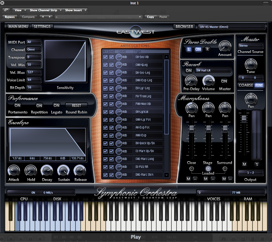
An example of keyswitches on a sampler can be seen in Figure 8.16. Some sampler systems even have intelligent playback that switch articulations automatically depending on how notes overlap or are played in relation to each other. The more articulations the system has, the better for getting realistic sound and range from an instrument,. However, knowing how and when to employ those articulations is often limited by your familiarity with the particular instrument, so musical experience plays an important role here.

[aside]In addition to the round-robin and multiple articulation samples, some instruments also include release samples, such as the subtle sound of a string being released or muted, which are played back when a note is released to help give it a natural and realistic ending.  Even these release samples could have round-robin variations of their own![/aside]

As you can see, realistic computer-generated music depends not only on the quality, but also the quantity and diversity of the content to play back. Realistic virtual instruments demand powerful and intelligent sampler playback systems, not to mention the computer hardware specs to support them. One company’s upright bass instrument alone contains over 21,000 samples. For optimum performance, some of these larger sampler systems even allow networked playback, out-sourcing the CPU and memory load of samples to other dedicated computers.

With the power and scope of the virtual instruments emerging today, it’s possible to produce full orchestral scores from your DAW. As nice as these virtual instruments are, they will only get you so far without additional production skills that help you get the most out of your digital compositions.

With the complexity of and diversity of the instruments that you’ll attempt to perform on a simple MIDI keyboard, it may take several passes at individual parts and sections to capture a performance you’re happy with. With MIDI, of course, merging performances and editing out mistakes is a simple task. It doesn’t require dozens of layers of audio files, messy crossfades, and the inherent issues of recorded audio. You can do as many takes as necessary and break down the parts in whatever way that helps to improve the performance.

[aside]In addition to the round-robin and multiple articulation samples, some instruments also include release samples, such as the subtle sound of a string being released or muted, which are played back when a note is released to help give it a natural and realistic ending.  Even these release samples could have round-robin variations of their own![/aside]

If your timing is inconsistent between performances, you can always quantize the notes. Quantization in MIDI refers to adjusting the performance data to the nearest selectable time value, be it whole note, half note, quarter note, etc. While quantizing can help tighten up your performance, it is also a main contributor to your composition sounding mechanical and unnatural. While you don’t want to be off by a whole beat, tiny imperfections in timing is natural with human performance and can help your music sound more convincing. Some DAW sequencers in addition to a unit of timing will let you choose a degree of quantization, in other words how forceful do you want to be when pushing your note data toward that fixed value. This will let you maintain some of the feel of your actual performance.

Most sequencers also have a collection of other MIDI processing functions – e.g., randomization. You can select a group of notes that you’ve quantized, and tell it to randomize the starting position and duration of the note (as well as other parameters such as note velocity) by some small amount, introducing some of these timing imperfections back into the performance. These processes are ironically sometimes known as humanization functions, which nevertheless can come in handy when polishing up a digital music composition.

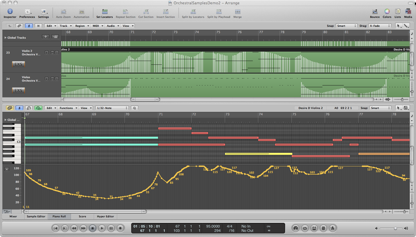
When actual musicians play their instruments, particularly longer sustained notes, they typically don’t play them at a constant level and timbre. They could be doing this in response to a marking of dynamics in the score (such as a crescendo), or they may simply be expressing their own style and interpretation of the music. Differences in the way notes are played also result from simple human factors. One trumpet player pushes the air a little harder than another to get a note started or to end a long note when he’s running out of breath. The bowing motion on a stringed instrument varies slightly as the bow moves back and forth, and differs from one musician to another. Only a machine can produce a note in exactly the same way every time. These nuances aren’t captured in timing or note velocity information, but some samplers can respond to MIDI control data in order to achieve these more dynamic performances. As the name might imply, an important one of these is MIDI controller 11, expression. Manipulating the expression value is a great way to add a natural, continuous arc to longer sustained notes, and it’s a great way to simulate dynamic swells as well as variations in string bowing. In many cases, controller 11 simply affects the volume of the playback, although some samplers are programmed to respond to it in a more dynamic way. Many MIDI keyboards have an expression pedal input, allowing you to control the expression with a variable foot pedal. If your keyboard has knobs or faders, you can also set these to write expression data, or you can always draw it in to your sequencer software by hand with a mouse or track pad.

An example of expression data captured into a MIDI sequencer region can be seen in Figure 8.17. MIDI controller 1, the modulation wheel, is also often linked to a variable element of the sampler instrument. In many cases, it will default as a vibrato control for the sound, either by applying a simple LFO to the pitch, or even dynamically crossfading with a recorded vibrato sample. When long sustained notes are played or sung live, a note pitch may start out normally, but, as the note goes on, an increasing amount of vibrato may be applied, giving it a nice fullness. Taking another pass over your music performance with the modulation wheel in hand, you can bring in varying levels of vibrato at appropriate times, enhancing the character and natural feel of your composition.

[wpfilebase tag=file id=142 tpl=supplement /]

As you can see, getting a great piece of music out of your digital composition isn’t always as simple as playing a few notes on your MIDI keyboard.  With all of the nuanced control available in today’s sampler systems, crafting even a single instrument part can require careful attention to detail and is often an exercise in patience.  Perhaps hiring a live musician is sounding much better at the moment?  Certainly, when you have access to the real deal, it is often a simpler and more effective way to create a piece of music.  Yet if you enjoy total control over their production and are deeply familiar and experienced with your digital music production toolset, virtual instruments can be a fast and powerful means of bringing your music to life.

8.2.3.1 Overdubbing

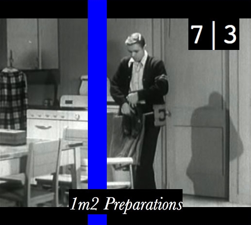
Post-production for film and video often requires a process of overdubbing.  Overdubbing production audio is referred to as ADR, which stands for Automated Dialog Replacement or Additional Dialogue Recording (depending on who you ask).   During this process, an actor is brought in to a recording studio, looks at the scene that was filmed during the production process, and listens to the performance she gave. The actor then attempts to recreate that performance vocally. Overdubbing is typically done in small chunks in a loop so the actor has multiple attempts to get it right. She’s trying to recreate not only the sound but also the speed of the original performance so that the new recording is synchronized with the movement of the lips on the screen. System clicks and streamers can be used to help the actor. Clicks (sometimes called beeps) are a rhythmic sound, like a metronome, that counts down to a certain point when the actor needs to start or hit a particular word. Streamers are a visual reference that follows the same speed of the clicks. The streamer is a solid line across the screen that moves in time with the clicks so you can see when important synchronization events occur. Clicks and streamers are also used in other post-production audio tasks for synchronizing sound effects and music during recording sessions. A click refers to a metronome that the conductor and musicians listen to do keep the music in time with the picture. A streamer is a colored vertical line that moves across the screen over a period of 2 to 4 seconds. When the streamer reaches the end of the screen the music is meant to reach a certain point. For example, the beginning of each measure might need to synchronize with the switch in the camera shot.

8.2.3.2 Mixing

Mixing is the process multiple sounds recorded on different tracks in a DAW are combined, with adjustments made to their relative levels, frequency components, dynamics, and special effects.  Then the resulting mix is channeled to different speakers appropriately.  The mixing process, hardware, and software were covered in detail in Chapter 7.  Thus, we focus here on practical and design considerations that direct the mixing process.

When you sit down to mix a recording you go through a process of trying to balance how you want the recording to sound against the quality of the recording. Often you will be limited in what you’re able to achieve with the mix because the source recording does not allow you sufficient manipulation. For example, if your recording of a band playing a song was recorded using a single overhead microphone, your ability to mix that recording is severely limited because all the instruments, room acoustic, and background noise are on the same track. You can turn the whole thing up or down, EQ and compress the overall recording, and add some reverb, but you have no control over the balance between the different instruments. On the other end of the spectrum you could have a recording with each instrument, voice, and other elements on separate tracks recording with separate microphones that were well-isolated from each other. In this scenario you have quite a bit of control over the mix, but mixing down 48 or more tracks is very time consuming. If you don’t have the time or expertise to harness all of that data, you may be forced to settle for something less than what you envision for the mix. Ultimately, you could work on a mix for the rest of your life and never be completely satisfied. So make sure you have clear goals and priorities for what you want to achieve with the mix and work through each priority until you run out of time or run out of parameters to manipulate.

Mixing sound for film or video can be particularly challenging because there are often quite a few different sounds happening at once. One way of taming the mix is to use surround sound. Mixing the various elements to different loudspeakers separates the sound such that each can be heard in the mix. Voices are typically mixed to the center channel, while music and sound effects are mixed to the four different surround channels. Loudness and dynamics are also an issue that gets close attention in the mixing process. In some cases you may need to meet a specific average loudness level over the course of the entire video. In other cases, you might need to compress the voices but leave the rest of the mix unchanged. The mix engineer will typically create stems (similar to busses or groups) to help with the process, such as a vocal stem, a music stem, and a sound effects stem. These stems can then be manipulated for various delivery mediums. You can see the usefulness of stems in situations where the sound being mixed is destined for one medium – for television broadcast as well as DVD distribution, for example.  The audio needs of a television broadcast are very different from the needs of a DVD. If the mix is ultimately going to be adjusted for both of these media, it is much easier to use stems rather returning to the original multitrack source, which may involve several hundred tracks.

 

8.2.3.3 Mastering

When you’ve completed the mixing process for a recording project, the next step is mastering the mixed-down audio. Mastering is the process of adjusting the dynamics and frequency response of a mix in order to optimize it for listening in various environments and prepare it for storage on the chosen medium. The term mastering comes from the idea of a master copy from which all other copies are made. Mastering is a particularly important step for music destined for CD or DVD, ensuring consistent levels and dynamics from one song to the next in an album.

In some ways you could describe the mastering process as making the mix sound louder. When mixing a multitrack recording, one thing you watch for is clipped signals. Once the mix is completed, you may have a well-balanced mix, but overall the mix sounds quieter than other mixes you hear on commercial recordings. What is typically happening is that you have one instrument in your mix that is a bit more dynamic than the others, and in order to keep the mix from clipping, you have to turn everything down because of this one instrument. One step in the mastering process is to use a multi-band compressor to address this problem.

A multi-band compressor is a set of compressors each of which operates on a limited frequency band without affecting others. A traditional compressor attenuates the entire mix when one frequency exceeds the threshold. A multi-band compressor, on the other hand, attenuates an instrument that is dynamic in one frequency band without attenuating other bands. This is often much more effective than using a simple EQ because the processing is only applied when needed, whereas an EQ will boost or cut a certain range of frequencies all the time. This allows you to let the less-dynamic frequencies take a more prominent role in the mix, resulting in the entire mix sounding louder.

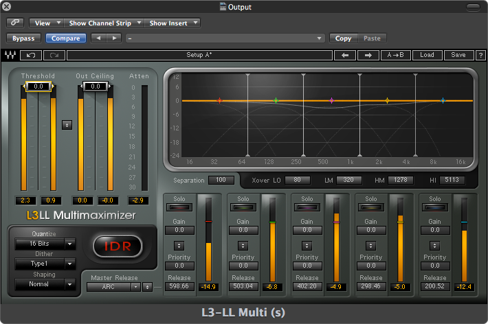
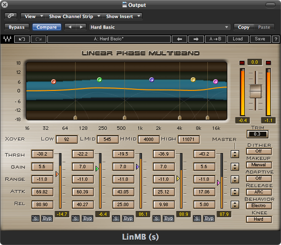
Figure 8.19 shows an example of a multi-band compressor with five separate bands of compression centered on the frequency indicated by the colored dots. You can set a separate threshold, gain, and compression range. In this case, a range is taking place of a ratio. The idea is that you want to compress the frequency band to stay within a given range. As you adjust the gain for each band, that range gets shifted up or down. This has the effect of manipulating the overall frequency response of the track in a way that is responsive to the changing amplitudes of the various frequencies. For example, if the frequency band centered at 1.5 kHz gets suddenly very loud, it can be attenuated for that period of time but then restored when the sound in that band drops back down to a more regular level.

You may also choose to apply some overall EQ in the mastering process to suit your taste. In some cases you may also manipulate the stereo image a bit to widen or narrow the overall stereo effect. You may also want to add a multi-band limiter at the end of the processing chain to catch any stray clipped signals that may have resulted from your other processes. If you’re converting to a lower bit depth, you should also apply a dither process to the mix to account for any quantization errors. For example, CDs require 16-bit samples, but most recording systems use 24 bits. Even if you are not converting bit depth you may still want to use dither since most DAW programs process the audio internally at 32 or 64 bits before returning back the original 24 bits. A 24-bit dither could help you avoid any quantization errors that would occur in that process. Figure 8.20 shows an example of a multi-band limiter that includes a dither processor.