6.2.1 Linking Controllers, Sequencers, and Synthesizers
In this section, we’ll look at how MIDI is handled in practice.
First, let’s consider a very simple scenario where you’re generating electronic music in a live performance. In this situation, you need only a MIDI controller and a synthesizer. The controller collects the performance information from the musician and transmits that data to the synthesizer. The synthesizer in turn generates a sound based on the incoming control data. This all happens in real-time, the assumption being that there is no need to record the performance.
Now suppose you want also want to capture the musician’s performance. In this situation, you have two options. The first option involves setting up a microphone and making an audio recording of the sounds produced by the synthesizer during the performance. This option is fine assuming you don’t ever need to change the performance, and you have the resources to deal with the large file size of the digital audio recording.
The second option is simply to capture the MIDI performance data coming from the controller. The advantage here is that the MIDI control messages constitute much less data than the data that would be generated if a synthesizer were to transform the performance into digital audio. Another advantage to storing in MIDI format is that you can go back later and easily change the MIDI messages, which generally is a much easier process than digital audio processing. If the musician played a wrong note, all you need to do is change the data byte representing that note number, and when the stored MIDI control data is played back into the synthesizer, the synthesizer generates the correct sound. In contrast, there’s no easy way to change individual notes in a digital audio recording. Pitch correction plug-ins can be applied to digital audio, but they potentially distort your sound, and sometimes can’t fix the error at all.
So let’s say you go with option two. For this, you need a MIDI sequencer between the controller and the synthesizer. The sequencer captures the MIDI data from the controller and sends it on to the synthesizer. This MIDI data is stored in the computer. Later, the sequencer can recall the stored MIDI data and send it again to the synthesizer, thereby perfectly recreating the original performance.
The next questions to consider are these: Which parts of this setup are hardware and which are software? And how do these components communicate with each other? Four different configurations for linking controllers, sequencers, and synthesizers are diagrammed in Figure 6.28. We’ll describe each of these in turn.
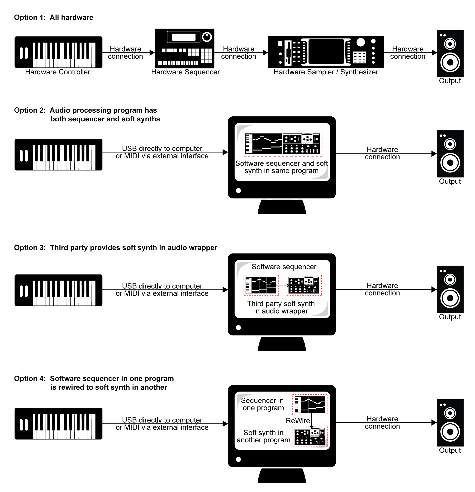
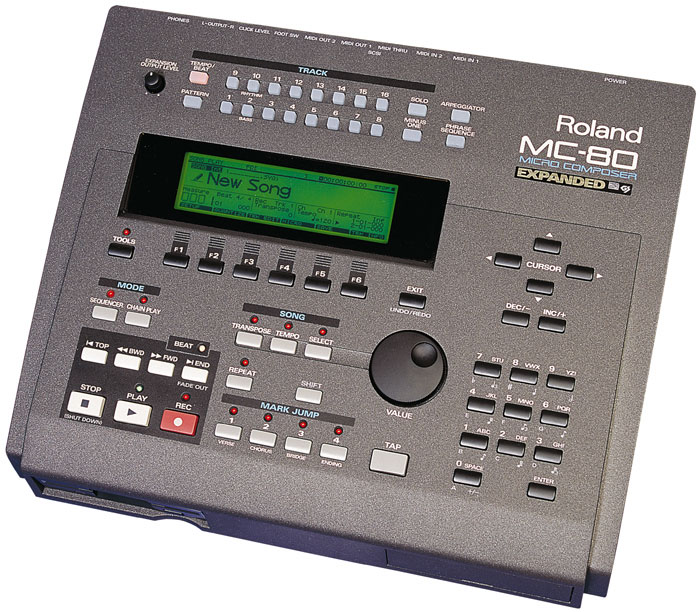
In the early days of MIDI, hardware synthesizers were the norm, and dedicated hardware sequencers also existed, like the one shown in Figure 6.29. Thus, an entire MIDI setup could be accomplished through hardware, as diagrammed in Option 1 of Figure 6.28.
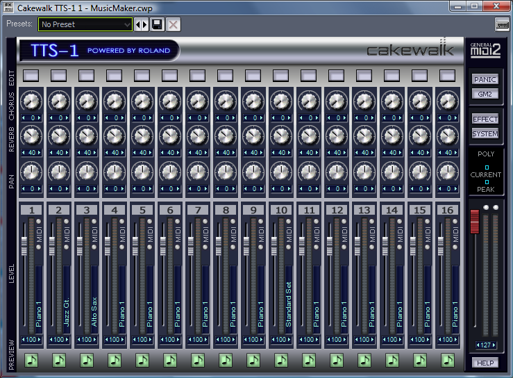
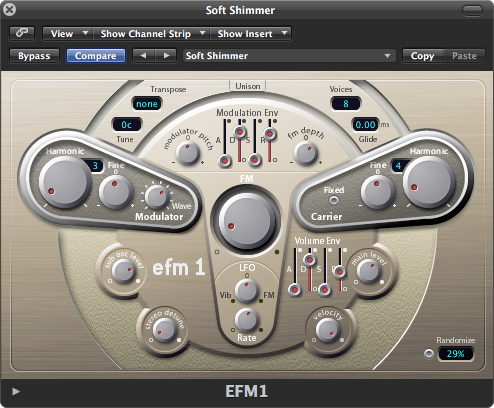
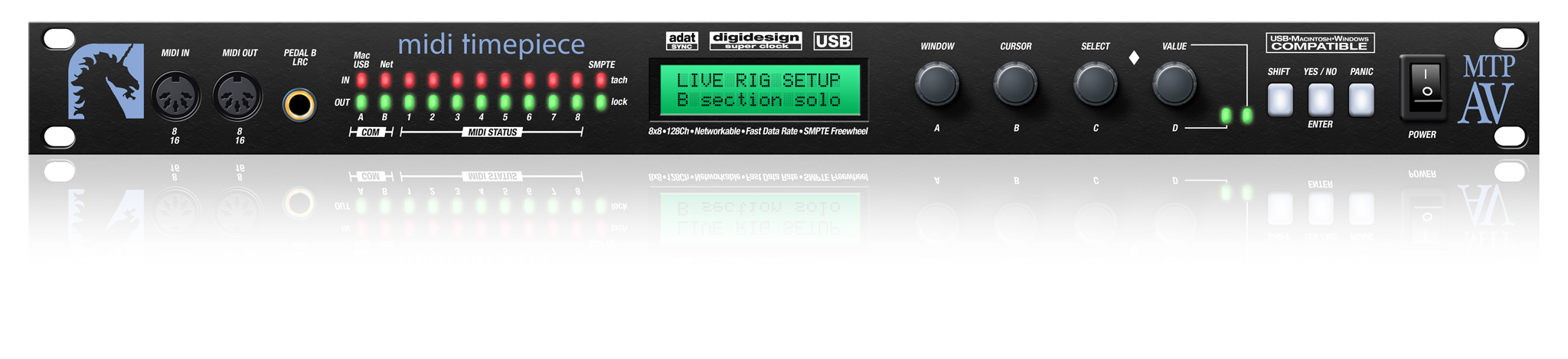
Now that personal computers have ample memory and large external drives, software solutions are more common. A standard setup is to have a MIDI controller keyboard connected to your computer via USB or through a USB MIDI interface like the one shown in Figure 6.30. Software on the computer serves the role of sequencer and synthesizer. Sometimes one program can serve both roles, as diagrammed in Option 2 of Figure 6.28. This is the case, for example, with both Cakewalk Sonar and Apple Logic, which provide a sequencer and built-in soft synths. Sonar’s sample-based soft synth is called the TTS, shown in Figure 6.31. Because samplers and synthesizers are often made by third party companies and then incorporated into software sequencers, they can be referred to as plug-ins. Logic and Sonar have numerous plug-ins that are automatically installed – for example, the EXS24 sampler (Figure 6.32) and the EFM1 FM synthesizer (Figure 6.33).


[aside]As you work with MIDI and digital audio, you’ll develop a large vocabulary of abbreviations and acronyms. In the area of plug-ins, the abbreviations relate to standardized formats that allow various software components to communicate with each other. VSTi stands for virtual studio technology instrument, created and licensed by Steinberg. This is one of the most widely used formats. Dxi is a plug-in format based on Microsoft Direct X, and is a Windows-based format. AU, standing for audio unit, is a Mac-based format. MAS refers to plug-ins that work with Digital Performer, an audio/MIDI processing system created by the MOTU company. RTAS (Real-Time AudioSuite) is the protocol developed by Digidesin for Pro Tools. You need to know which formats are compatible on which platforms. You can find the most recent information through the documentation of your software or through on-line sources.[/aside]
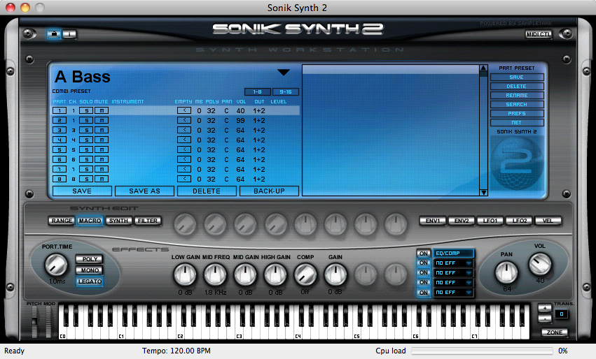
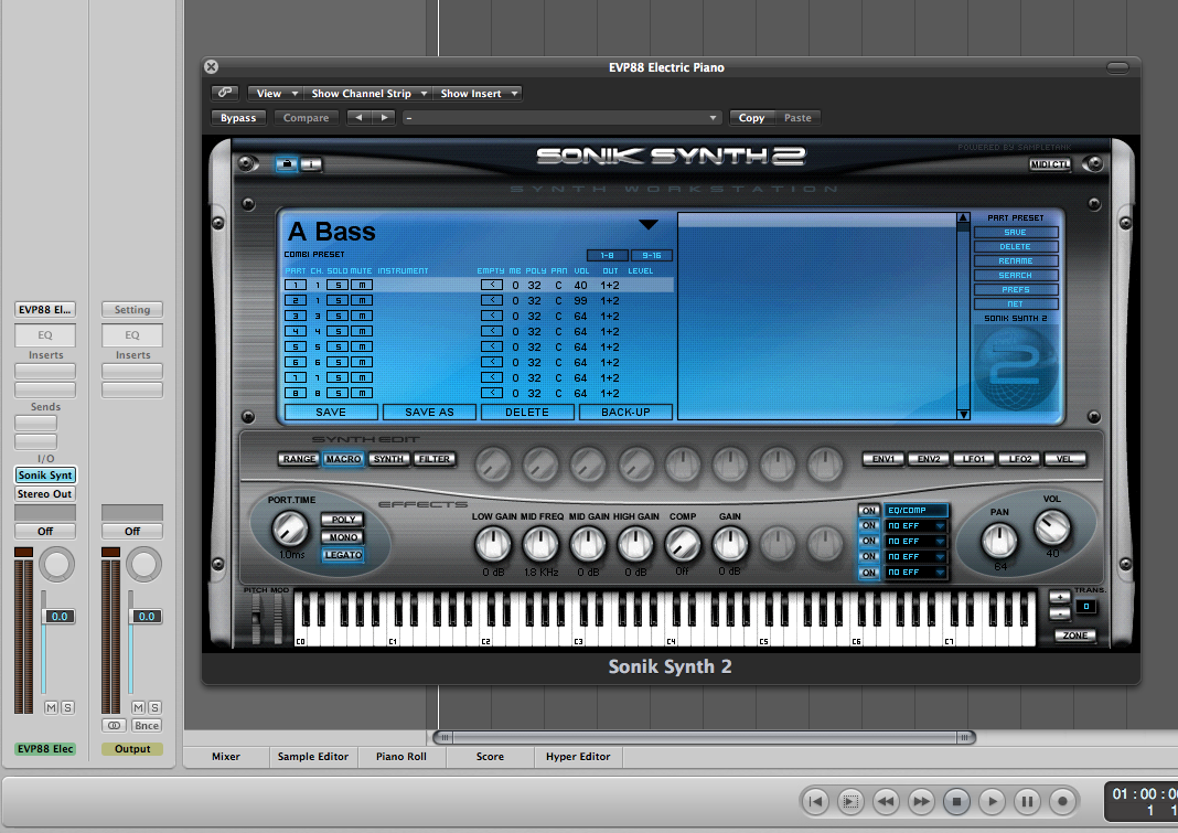
Some third-party vendor samplers and synthesizers are not automatically installed with a software sequencer, but they can be added by means of a software wrapper. The software wrapper makes it possible for the plug-in to run natively inside the sequencer software. This way you can use the sequencer’s native audio and MIDI engine and avoid the problem of having several programs running at once and having to save your work in multiple formats. Typically what happens is a developer creates a standalone soft synth like the one shown in Figure 6.34. He can then create an Audio Unit wrapper that allows his program to be inserted as an Audio Unit instrument, as shown for Logic in Figure 6.35. He can also create a VSTi wrapper for his synthesizer that allows the program to be inserted as a VSTi instrument in a program like Cakewalk, an MAS wrapper for MOTU Digital Performer, and so forth. A setup like this is shown in Option 3 of Figure 6.28.
An alternative to built-in synths or installed plug-ins is to have more than one program running on your computer, each serving a different function to create the music. An example of such a configuration would be to use Sonar or Logic as your sequencer, and then use Reason to provide a wide array of samplers and synthesizers. This setup introduces a new question: How do the different software programs communicate with each other?
One strategy is to create little software objects that pretend to be MIDI or audio inputs and outputs on the computer. Instead of linking directly to input and output hardware on the computer, you use these software objects as virtual cables. That is, the output from the MIDI sequencer program goes to the input of the software object, and the output of the software object goes to the input of the MIDI synthesis program. The software object functions as a virtual wire between the sequencer and synthesizer. The audio signal output by the soft synth can be routed directly to a physical audio output on your hardware audio interface, to a separate audio recording program, or back into the sequencer program to be stored as sampled audio data. This configuration is diagrammed in Option 4 of Figure 6.28.
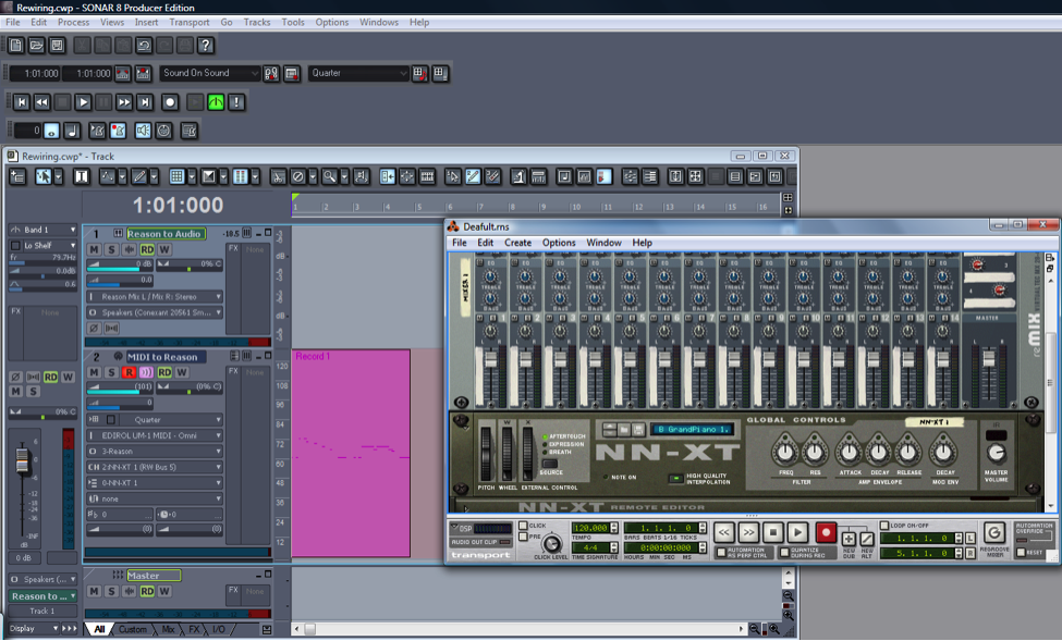
An example of this virtual wire strategy is the Rewire technology developed by Propellerhead and used with its sampler/synthesizer program, Reason. Figure 6.36 shows how a track in Sonar can be rewired to connect to a sampler in Reason. The track labeled “MIDI to Reason” has the MIDI controller as its input and Reason as its output. The NN-XT sampler in Reason translates the MIDI commands into digital audio and sends the audio back to the track labeled “Reason to audio.” This track sends the audio output to the sound card.
Other virtual wiring technologies are available. Soundflower is another program for Mac OS X developed by Cycling ’74 that creates virtual audio wires that can be routed between programs. CoreMIDI Virtual Ports are integrated into Apple’s CoreMIDI framework on Mac OS X. A similar technology called MIDI Yoke (developed by a third party) works in the Windows operating systems. Jack is an open source tool that runs on Windows, Mac OS X, and various UNIX platforms to create virtual MIDI and audio objects.
6.2.2 Creating Your Own Synthesizer Sounds
[wpfilebase tag=file id=25 tpl=supplement /]
[wpfilebase tag=file id=43 tpl=supplement /]
Section 6.1.8 covered the various components of a synthesizer. Now that you’ve read about the common objects and parameters available on a synthesizer you should have an idea of what can be done with one. So how do you know which knobs to turn and when? There’s not an easy answer to that question. The thing to remember is that there are no rules. Use your imagination and don’t be afraid to experiment. In time, you’ll develop an instinct for programming the sounds you can hear in your head. Even if you don’t feel like you can create a new sound from scratch, you can easily modify existing patches to your liking, learning to use the controls along the way. For example, if you load up a synthesizer patch and you think the notes cut off too quickly, just increase the release value on the amplitude envelope until it sounds right.
Most synthesizers use obscure values for the various controls, in the sense that it isn’t easy to relate numerical settings to real-world units or phenomena. Reason uses control values from 0 to 127. While this nicely relates to MIDI data values, it doesn’t tell you much about the actual parameter. For example, how long is an attack time of 87? The answer is, it doesn’t really matter. What matters is what it sounds like. Does an attack time of 87 sound too short or too long? While it’s useful to understand what the controller affects, don’t get too caught up in trying to figure out what exact value you’re dialing in when you adjust a certain parameter. Just listen to the sound that comes out of the synthesizer. If it sounds good, it doesn’t matter what number is hiding under the surface. Just remember to save the settings so you don’t lose them.
[separator top=”0″ bottom=”1″ style=”none”]
6.2.3 Making and Loading Your Own Samples
[wpfilebase tag=file id=23 tpl=supplement /]
Sometimes you may find that you want a certain sound that isn’t available in your sampler. In that case, you may want to create your own sample
If you want to create a sampler patch that sounds like a real instrument, the first thing to do is find someone who has the instrument you’re interested in and get them to play different notes one at a time while you record them. To make sure you don’t have to stretch the pitch too far for any one sample, make sure you get a recording for at least three notes per octave within the instrument’s range.
[wpfilebase tag=file id=136 tpl=supplement /]
Keep in mind that the more samples you have, the more RAM space the sampler requires. If you have 500 MB worth of recorded samples and you want to use them all, the sampler is going to use up 500 MB of RAM on your computer. The trick is finding the right balance between having enough samples so that none of them get stretched unnaturally, but not so many that you use up all the RAM in your computer. As long as you have a real person and a real instrument to record, go ahead and get as many samples as you can. It’s much easier to delete the ones you don’t need than to schedule another recording session to get the two notes you forgot to record.Some instruments can sound different depending on how they are played. For example, a trumpet sounds very different with a mute inserted on the horn. If you want your sampler to be able to create the muted sound, you might be able to mimic it using filters in the sampler, but you’ll get better results by just recording the real trumpet with the mute inserted. Then you can program the sampler to play the muted samples instead of the unmuted ones when it receives a certain MIDI command.
Once you have all your samples recorded, you need to edit them and add all the metadata required by the sampler. In order for the sampler to do what it needs to do with the audio files, the files need to be in an uncompressed file format. Usually this is WAV or AIF format. Some samplers have a limit on the sampling rate they can work with. Make sure you convert the samples to the rate required by the sampler before you try to use them.
[wpfilebase tag=file id=137 tpl=supplement /]
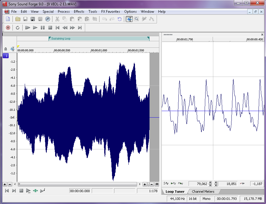
Figure 6.37 shows a loop defined in a sample editing program. On the left side of the screen you can see the overall waveform of the sample, in this case a violin. In the time ruler above the waveform you can see a green bar labeled Sustaining Loop. This is the portion of the sample that is looped. On the right side of the screen you can see a close up view of the loop point. The left half of the wave is the end of the sample, and the right part of the wave is the start of the loop point. The trick here is to line up the loop points so the two parts intersect with the zero amplitude cross point. This way you avoid any clicks or pops that might be introduced when the sampler starts looping the playback.The first bit of metadata you need to add to each sample is a loop start and loop end marker. Because you’re working with prerecorded sounds, the sound doesn’t necessarily keep playing just because you’re still holding the key down on the keyboard. You could just record your samples so they hold on for a long time, but that would use up an unnecessary amount of RAM. Instead, you can tell the sampler to play the file from the beginning and stop playing the file when the key on the keyboard is released. If the key is still down when the sampler reaches the end of the file, the sampler can start playing a small portion of the sample over and over in an endless loop until the note is released. The challenge here is finding a portion of the sample that loops naturally without any clicks or other swells in amplitude or harmonics.
In some sample editors you can also add other metadata that saves you programming time later. For WAV and AIF files, you can add information about the root pitch of the sample and the range of notes this sample should cover. You can also add information about the loop behavior. For example, do you want the sample to continue to loop during the release of the amplitude envelope, or do you want it to start playing through to the end of the file? You could set the sample not to loop at all and instead play as a “one shot” sample. This means the sample ignores Note Off events and play the sample from beginning to end every time. Some samplers can read that metadata and do some pre-programming for you on the sampler when you load the sample.

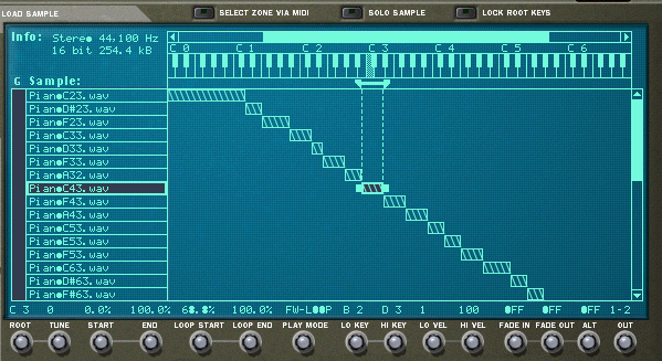
Once the samples are ready, you can load them into the sampler. If you weren’t able to add the metadata about root key and loop type, you’ll have to add that manually into the sampler for each sample. You’ll also need to decide which notes trigger each sample and which velocities each sample responds to. This process of assigning root keys and key ranges to all your samples is a time consuming but essential process. Figure 6.39 shows a list of sample WAV files loaded in a software sampler. In the figure we have the sample “PianoC43.wav” selected. You can see in the center of the screen the span of keys that have been assigned to that sample. Along the bottom row of the screen you can see the root key, loop, and velocity assignments for that sample.
Once you have all your samples loaded and assigned, each sample can be passed through a filter and amplifier which can in turn be modulated using envelopes, LFO, and MIDI controller commands. Most samplers let you group samples together into zones or keygroups allowing you to apply a single set of filters, envelopes, etc. This feature can save a lot of time in programming. Imagine programming all of those settings on each of 100 samples without losing track of how far you are in the process. Figure 6.40 shows all the common synthesizer objects being applied to the “PianoC43.wav” sample.

6.2.4 Data Flow and Performance Issues in Audio/MIDI Recording
Combined audio/MIDI recording can place high demands on a system, requiring a fast CPU and hard drive, an appropriate choice of audio driver, and a careful setting of the audio buffer size. These components affect your ability to record, process, and play sound, particularly in real time.
In Chapter 5, we introduced the subject of latency in digital audio systems. The problem of latency is compounded when MIDI data is added to the mix. A common frustration in MIDI recording sessions is that there can be an audible difference between the moment when you press a key on a MIDI controller keyboard and the moment when you hear the sound coming out of the headphones or monitors. In this case, the latency is the result of your buffer size. The MIDI signal generated by the key press must be transformed into digital audio by a synthesizer or sampler, and the digital data is then placed in the output buffer. This sound is not heard until the buffer is filled up. When the buffer is full, it undergoes ADC and is set sent to the headphones or monitors. Playback latency results when the buffer is too large. As discussed in Chapter 5, you can reduce the playback latency by using a low latency audio driver like ASIO or reducing the buffer size if this option is available in your driver. However, if you make the buffer size too low, you’ll have breaks in the sound when the CPU cannot keep up with the number of times it has to empty the buffer.
Another potential bottleneck in digital audio playback is the hard drive. Fast hard drives are a must when working with digital audio, and it is also important to use a dedicated hard drive for your audio files. If you’re storing your audio files on the same hard drive as your operating system, you’ll need a larger playback buffer to accommodate all the times the hard drive is busy delivering system data instead of your audio. If you get a second hard drive and use it only for audio files, you can usually get away with a much smaller playback buffer, thereby reducing the playback latency.
When you use software instruments, there are other system resources besides the hard drive that also become a factor to consider. Software samplers require a lot of system RAM because all the audio samples have to be loaded completely in RAM in order for them to be instantly accessible. On the other hand, software synthesizers that generate the sound dynamically can be particularly hard on the CPU. The CPU has to mathematically create the audio stream in real time, which is a more computationally intense process than simply playing an audio stream that already exists. Synthesizers with multiple oscillators can be particularly problematic. Some programs let you offload individual audio or instrument tracks to another CPU. This could be a networked computer running a processing node program or some sort of dedicated processing hardware connected to the host computer. If you’re having problems with playback dropouts due to CPU overload and you can’t add more CPU power, another strategy is to render the instrument audio signal to an audio file that is played back instead of generated live (often called “freezing” a track). However, this effectively disables the MIDI signal and the software instrument so if you need to make any changes to the rendered track, you need to go back to the MIDI data and re-render the audio. Check pdf2word.org/ for more tips.
6.2.5 Non-Musical Applications for MIDI
6.2.5.1 MIDI Show Control
MIDI is not limited to use for digital music. There have been many additions to the MIDI specification to allow MIDI to be used in other areas. One addition is the MIDI Show Control Specification. MIDI Show Control (MSC) is used in live entertainment to control sound, lighting, projection, and other automated features in theatre, theme parks, concerts, and more.
MSC is a subset of the MIDI Systems Exclusive (SysEx) status byte. MIDI SysEx commands are typically specific to each manufacturer of MIDI devices. Each manufacturer gets a SysEx ID number. MSC has a SysEx sub-ID number of 0x02. The syntax, in hexadecimal, for a MSC message is:
F0 7F <device_ID> 02 <command_format> <command> <data> F7
- F0 is the status byte indicating the start of a SysEx message.
- 7F indicates the use of a SysEx sub-ID. This is technically a manufacturer ID that has been reserved to indicate extensions to the MIDI specification.
- <device_ID> can be any number between 0x00 and 0x7F indicating the device ID of the thing you want to control. These device ID numbers have to be set on the receiving end as well so each device knows which messages to respond to and which messages to ignore. 0x7F is a universal device ID. All devices respond to this ID regardless of their individual ID numbers.
- 02 is the sub-ID number for MIDI Show Control. This tells the receiving device that the bytes that follow are MIDI Show Control syntax as opposed to MIDI Machine Control, MIDI Time Code, or other commands.
- <command_format> is a number indicating the type of device being controlled. For example, 0x01 indicates a lighting device, 0x40 indicates a projection device, and 0x60 indicates a pyrotechnics device. A complete list of command format numbers can be found in the MIDI Show Control 1.1 specification.
- <command> is a number indicating the type of command being sent. For example, 0x01 is “GO”, 0x02 is “STOP”, 0x03 is “RESUME”, 0x0A is “RESET”.
- <data> represents a variable number of data bytes that are required for the type of command being sent. A “GO” command might need some data bytes to indicate the cue number that needs to be executed from a list of cues on the device. If no cue number is specified, the device simply executes the next cue in the list. Two data bytes (0x00, 0x00) are still needed in this case as delimiters for the cue number syntax. Some MSC devices are able to interpret the message without these delimiters, but they’re technically required in the MSC specification.
- F7 is the End of Systems Exclusive byte indicating the end of the message.
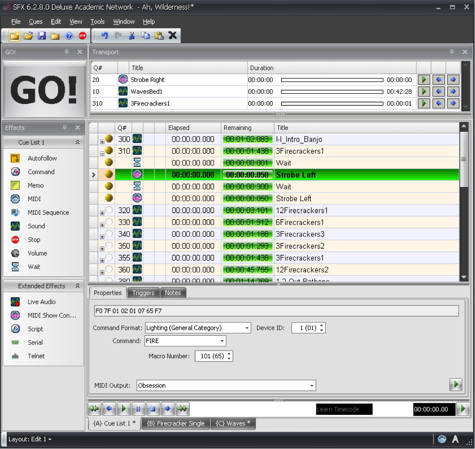
Most lighting consoles, projection systems, and computer sound playback systems used in live entertainment are able to generate and respond to MSC messages. Typically, you don’t have to create the commands manually in hex. You have a graphical interface that lets you choose the command you’re want from a list of menus. Figure 6.41 shows some MSC FIRE commands for a lighting console generated as part of a list of sound cues. In this case, the sound effect of a firecracker is synchronized with the flash of a strobe light using MSC.
6.2.5.2 MIDI Relays and Footswitches
You may not always have a device that knows how to respond to MIDI commands. For example, although there is a MIDI Show Control command format for motorized scenery, the motor that moves a unit on or off the stage doesn’t understand MIDI commands. However, it does understand a switch. There are many options available for MIDI controlled relays that respond to a MIDI command by making or breaking an electrical contact closure. This makes it possible for you to connect the wires for the control switch of a motor to the relay output, and then when you send the appropriate MIDI command to the relay, it closes the connection and the motor starts turning.
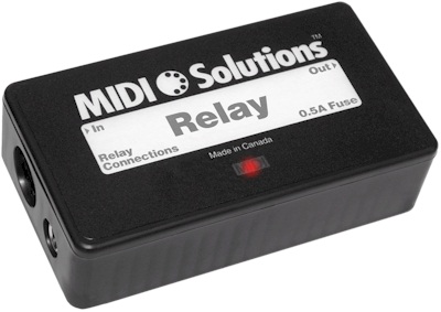
Another possibility is that you may want to use MIDI commands without a traditional MIDI controller. For example, maybe you want a sound effect to play each time a door is opened or closed. Using a MIDI footswitch device, you could wire up a magnetic door sensor to the footswitch input and have a MIDI command sent to the computer each time the door is opened or closed. The computer could then be programmed to respond by playing a sound file. Figure 6.42 shows an example of a MIDI relay device.
6.2.5.3 MIDI Time Code
MIDI sequencers, audio editors, and audio playback systems often need to synchronize their timeline with other systems. Synchronization could be needed for working with sound for video, lighting systems in live performance, and even automated theme park attractions. The world of filmmaking has been dealing with synchronization issues for decades, and the Society of Motion Picture and Television Engineers (SMPTE) has developed a standard format for a time code that can be used to keep video and audio in sync. Typically this is accomplished using an audio signal called Linear Time Code that has the synchronization data encoded in SMPTE format. The format is Hours:Minutes:Seconds:Frames. The number of frames per second varies, but the standard allows for 24, 25, 29.97 (also known as 30-Drop), and 30 frames per second.
MIDI Time Code (MTC) uses this same time code format, but instead of being encoded into an analog audio signal, the time information is transmitted in digital format via MIDI. A full MIDI Time Code message has the following syntax:
F0 7F <device_ID> <sub-ID 1> <sub-ID 2> <hr> <mn> <sc> <fr> F7
- F0 is the status byte indicating the start of a SysEx message.
- 7F indicates the use of a SysEx sub-ID. This is technically a manufacturer ID that has been reserved to indicate extensions to the MIDI specification.
- <device_ID> can be any number between 0x00 and 0x7F indicating the device ID of the thing you want to control. These device ID numbers have to be set on the receiving end as well so each device knows which messages to respond to and which messages to ignore. 0x7F is a universal device ID. All devices respond to this ID regardless of their individual ID numbers.
- <sub-ID 1> is the sub-ID number for MIDI Time Code. This tells the receiving device that the bytes that follow are MIDI Time Code syntax as opposed to MIDI Machine Control, MIDI Show Control, or other commands. There are a few different MIDI Time Code sub ID numbers. 01 is used for full SMPTE messages and for SMPTE user bits messages. 04 is used for a MIDI Cueing message that includes a SMPTE time along with values for markers such as Punch In/Out and Start/Stop points. 05 is used for real-time cuing messages. These messages have all the marker values but use the quarter-frame format for the time code.
- <sub-ID 2> is a number used to define the type of message within the sub-ID 1 families. For example, there are two types of Full Messages that use 01 for sub-ID 1. A value of 01 for sub-ID 2 in a Full Message would indicate a Full Time Code Message whereas 02 would indicate a User Bits Message.
- <hr> is a byte that carries both the hours value as well as the frame rate. Since there are only 24 hours in a day, the hours value can be encoded using the five least significant bits, while the next two greater significant bits are used for the frame rate. With those two bits you can indicate four different frame rates (24, 25, 29.97, 30). As this is a data byte, the most significant bit stays at 0.
- <mn> represents the minutes value 00-59.
- <sc> represents the seconds value 00-59.
- <fr> represents the frame value 00-29.
- F7 is the End of Systems Exclusive byte indicating the end of the message.
For example, to send a message that sets the current timeline location of every device in the system to 01:30:35:20 in 30 frames/second format, the hexadecimal message would be:
F0 7F 7F 01 01 61 1E 23 14 F7
Once the full message has been transmitted, the time code is sent in quarter-frame format. Quarter-frame messages are much smaller than full messages. This is less demanding of the system since only two bytes rather than ten bytes have to be parsed at a time. Quarter frame messages use the 0xF1 status byte and one data byte with the high nibble indicating the message type and the low nibble indicating the value of the given time field. There are eight message types, two for each time field. Each field is separated into a least significant nibble and a most significant nibble:
0 = Frame count LS
1 = Frame count MS
2 = Seconds count LS
3 = Seconds count MS
4 = Minutes count LS
5 = Minutes count MS
6 = Hours count LS
7 = Hours count MS and SMPTE frame rate
As the name indicates, quarter frame messages are transmitted in increments of four messages per frame. Messages are transmitted in the order listed above. Consequently, the entire SMPTE time is completed every two frames. Let’s break down the same 01:30:35:20 time value into quarter frame messages in hexadecimal. This time value would be broken up into eight messages:
F1 04  (Frame LS)
F1 11  (Frame MS)

F1 23  (Seconds LS)
F1 32  (Seconds MS)

F1 4E  (Minutes LS)
F1 51  (Minutes MS)

F1 61  (Hours LS)
F1 76  (Hours MS and Frame Rate)
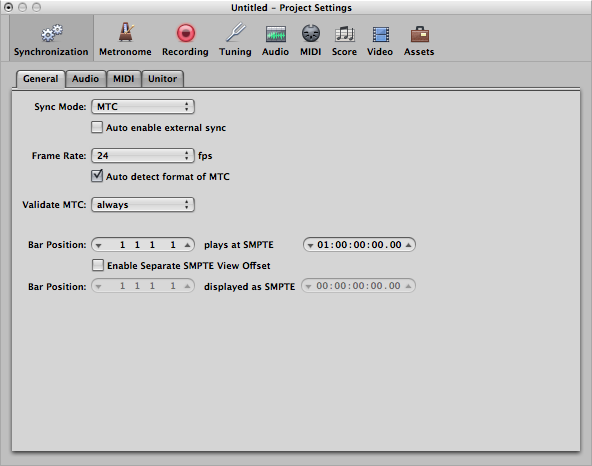
When synchronizing systems with MIDI Time Code, one device needs to be the master time code generator and all other devices need to be configured to follow the time code from this master clock. Figure 6.43 shows Logic Pro configured to synchronize to an incoming MIDI Time Code signal. If you have a mix of devices in your system that follow LTC or MTC, you can also put a dedicated time code device in your system that collects the time code signal in LTC or MTC format and then relay that time code to all the devices in your system in the various formats required, as shown in Figure 6.44.
6.2.5.4 MIDI Machine Control
[wpfilebase tag=file id=44 tpl=supplement /]
Another subset of the MIDI specification is a set of commands that can control the transport system of various recording and playback systems. Transport controls are things like play, stop, rewind, record, etc. This command set is called MIDI Machine Control. The specification is quite comprehensive and includes options for SMPTE time code values, as well as confirmation response messages from the devices being controlled. A simple MMC message has the following syntax:
F0 7F <device_ID> 06 <command> F7
- F0 is the status byte indicating the start of a SysEx message.
- 7F indicates the use of a SysEx sub-ID. This is technically a manufacturer ID that has been reserved to indicate extensions to the MIDI specification.
- <device_ID> can be any number between 0x00 and 0x7F indicating the device ID of the thing you want to control. These device ID numbers have to be set on the receiving end as well so each device knows which messages to respond to and which messages to ignore. 0x7F is a universal device ID. All devices respond to this ID regardless of their individual ID numbers.
- 06 is the sub-ID number for MIDI Machine Control. This tells the receiving device that the bytes that follow are MIDI Machine Control syntax as opposed to MIDI Show Control, MIDI Time Code, or other commands.
- <command> can be a set of bytes as small as one byte and can include several bytes communicating various commands in great detail. A simple play (0x02) or stop (0x01) command only requires a single data byte.
- F7 is the End of Systems Exclusive byte indicating the end of the message.
A MMC command for PLAY would look like this:
F0 7F 7F 06 02 F7
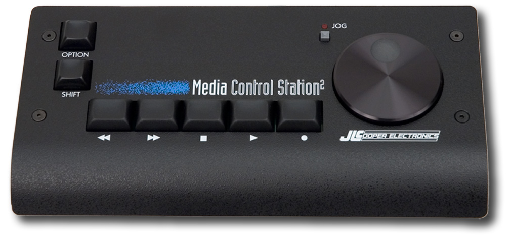
MIDI Machine Control was really a necessity when most studio recording systems were made up of several different magnetic tape-based systems or dedicated hard disc recorders. In these situations, a single transport control would make sure all the devices were doing the same thing. In today’s software-based systems, MIDI Machine Control is primarily used with MIDI control surfaces, like the one shown in Figure 6.45, that connect to a computer so you can control the transport of your DAW software without having to manipulate a mouse.