5.3.1 Reading and Writing Audio Files in MATLAB
A number of exercises in this book ask that you experiment with audio processing by reading an audio file into MATLAB or a C++ program, manipulate it in some way, and either listen directly to the result or write the result back to a file. In Chapter 2 we introduced how to read in WAV files in MATLAB. Let’s look at this in more detail now.
In some cases, you may want to work with raw audio data coming from an external source. One way to generate raw audio data is to take a clip of music or sound and, in Audacity or some other higher level tool, save or export the clip as an uncompressed or raw file. Audacity allows you to save in uncompressed WAV or AIFF formats (Figure 5.31).
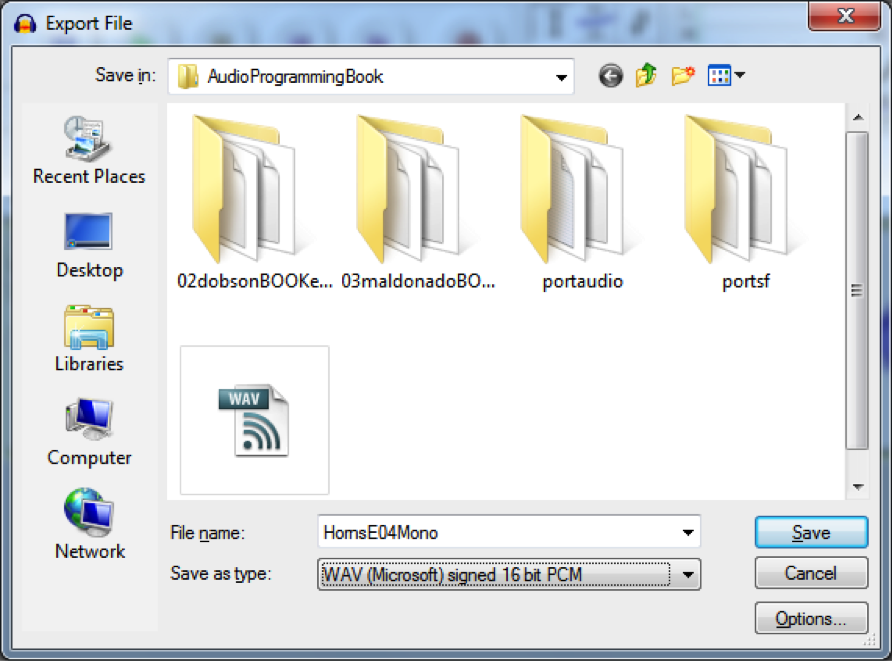
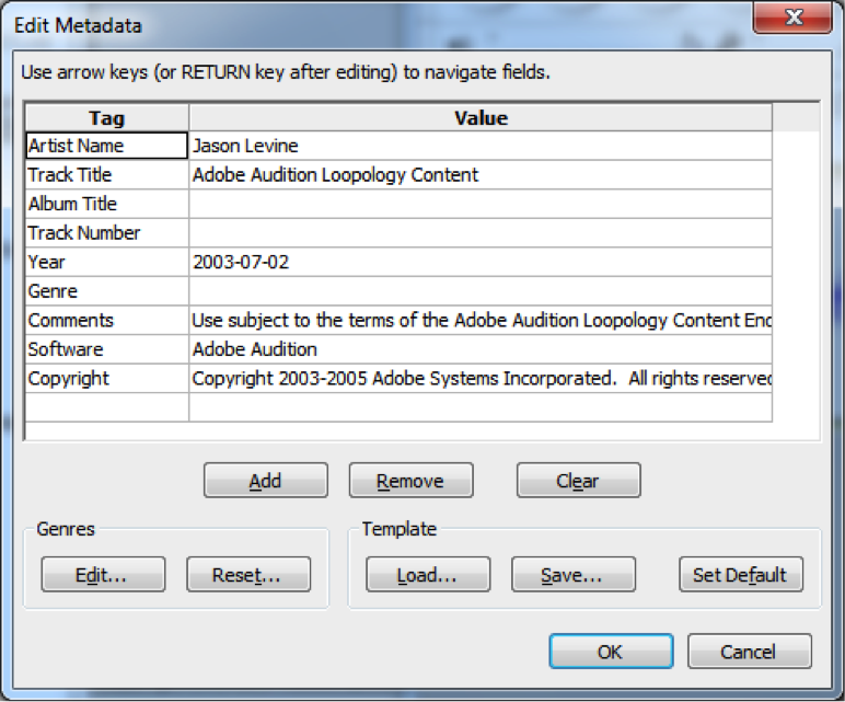
From the next input box that pops open, you can see that although this file is being saved as uncompressed PCM, it still has a WAV header on it containing metadata.
The WAV file can be read an array in MATLAB with the following:
xWav = audioread('HornsE04Mono.wav');
The audioread function strips the header off and places the raw audio values into the array x. These values have a maximum range from -1 to 1. If you want to know the sampling rate sr and bit depth b, you can use this:
[xWav, sr, b] = audioread('HornsE04Mono.wav');
If the file is stereo, you’ll get a two-dimensional array with the same number of samples in each channel.
Adobe Audition allows you to save an audio file as raw data with no header by deselecting the “Save extra non-audio information” box (Figure 5.33).

When you save a file in this manner, you need to remember the sampling rate and bit depth. A raw audio file is read in MATLAB as follows:
fid = fopen('HornsE04Mono.raw', 'r');
xRaw16 = fread(fid, 'int16');
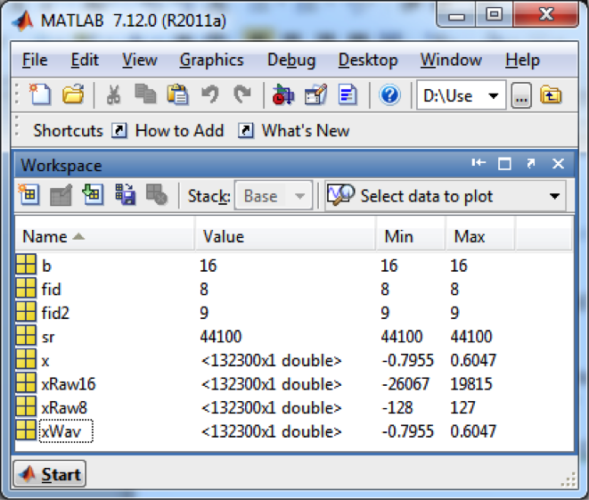
fid is the file handle, and the r in single quotes means that the file is being opened to be read. The type specifier int16 is used in fread so that MATLAB knows to interpret the input as 16-bit signed integers. MATLAB’s workspace window should show you that the values are in the maximum range of -32768 to 32767 ($$-2^{b-1}\: to\: 2^{b-1}-1$$) (Figure 5.34). The values don’t span the maximum range possible because they were at low amplitude to begin with.
For HornsE04Mono_8bits.raw, an 8-bit file, you can use
fid2 = fopen('HornsE04Mono_8bits.raw', 'r');
xRaw8 = fread(fid2, 'int8');
The values of xRaw8 range from -128 to 127, as shown in Figure 5.34.
A stereo RAW file has twice as many samples as the corresponding mono file, with the samples for the two stereo channels interleaved.
You can use the fwrite function in MATLAB to write the file back out to permanent storage after you’ve manipulated the values.
5.3.2 Raw Audio Data in C++
[wpfilebase tag=file id=91 tpl=supplement /]
In Chapters 2 and 3, we showed you how to generate sinusoidal waveforms as arrays of values that could be sent directly to the sound device and played. But what if you want to work with more complicated sounds and music in C++? In this case, you’ll need to be able to read audio files into your programs in order to experiment with audio processing.
In C++, raw audio data in 8-bit or 16-bit format can be read into an array of characters (char) or short integers (short), respectively, assuming that characters are stored in 8 bits and short integers are 16 bits on your system. This is demonstrated in Program 5.1. You can use this in the programming exercise on dithering and mu-law encoding.
//This program runs under OSS
//The program expects an 8-bit raw sound file.
//You can alter it to read a 16-bit file into short ints
#include <sys/ioctl.h> //for ioctl()
#include <math.h> //sin(), floor()
#include <stdio.h> //perror
#include <fcntl.h> //open
#include <linux/soundcard.h> //SOUND_PCM*
#include <stdlib.h>
#include <unistd.h>

using namespace std;

#define TYPE char
#define RATE 44100 //sampling rate
#define SIZE sizeof(TYPE) //size of sample, in bytes
#define CHANNELS 1 //number of stereo channels
#define PI 3.14159
#define SAMPLE_MAX (pow(2,SIZE*8 - 1) - 1)

void writeToSoundDevice(TYPE* buf, int deviceID, int buffSize) {
  int status;
  status = write(deviceID, buf, buffSize);
  if (status != buffSize)
    perror("Wrote wrong number of bytes\n");
  status = ioctl(deviceID, SOUND_PCM_SYNC, 0);
  if (status == -1)
    perror("SOUND_PCM_SYNC failed\n");
}

int main(int argc, char* argv[])
{
  int deviceID, arg, status, i, numSamples;
  numSamples = atoi(argv[1]);

  TYPE* samples = (TYPE *) malloc((size_t) numSamples * sizeof(TYPE)* CHANNELS);
  FILE *inFile = fopen(argv[2], "rb");
  fread(samples, (size_t)sizeof(TYPE), numSamples*CHANNELS, inFile);
  fclose(inFile);

  deviceID = open("/dev/dsp", O_WRONLY, 0);
  if (deviceID < 0)
    perror("Opening /dev/dsp failed\n");
  arg = SIZE * 8;
  status = ioctl(deviceID, SOUND_PCM_WRITE_BITS, &arg);
  if (status == -1)
    perror("Unable to set sample size\n");
  arg = CHANNELS;
  status = ioctl(deviceID, SOUND_PCM_WRITE_CHANNELS, &arg);
  if (status == -1)
    perror("Unable to set number of channels\n");
  arg = RATE;
  status = ioctl(deviceID, SOUND_PCM_WRITE_RATE, &arg);
  if (status == -1)
    perror("Unable to set number of bits\n");

  writeToSoundDevice(samples, deviceID, numSamples * CHANNELS);
  FILE *outFile = fopen(argv[3], "wb");
  fwrite(samples, 1, numSamples*CHANNELS, outFile);
  fclose(outFile);
  close(deviceID);
}
Program 5.1 Reading raw data in a C++ program, OSS library
When you write a low-level sound program such as this, you need to use a sound library such as OSS or ALSA. There’s a lot of documentation online that will guide you through installation of the sound libraries into the Linux environment and show you how to program with the libraries. (See the websites cited in the references at the end of the chapter.) The ALSA version of Program 5.1 is given in Program 5.2.
/*This program demonstrates how to read in a raw
  data file and write it to the sound device to be played.
  The program uses the ALSA library.
  Use option -lasound on compile line.*/

#include </usr/include/alsa/asoundlib.h>
#include <math.h>
#include <iostream>
using namespace std;

static char *device = "default";	/*default playback device */
int main(int argc, char* argv[])
{
  int err, numSamples;
  snd_pcm_t *handle;
  snd_pcm_sframes_t frames;
  numSamples = atoi(argv[1]);
  char* samples = (char*) malloc((size_t) numSamples);
  FILE *inFile = fopen(argv[2], "rb");
  int numRead = fread(samples, 1, numSamples, inFile);
  fclose(inFile);
if ((err=snd_pcm_open(&handle, device, SND_PCM_STREAM_PLAYBACK, 0)) < 0){
    printf("Playback open error: %s\n", snd_strerror(err));
    exit(EXIT_FAILURE);
  }
if ((err =
 snd_pcm_set_params(handle,SND_PCM_FORMAT_U8,
   SND_PCM_ACCESS_RW_INTERLEAVED,1,44100, 1, 100000) ) < 0 ){
        printf("Playback open error: %s\n", snd_strerror(err));
        exit(EXIT_FAILURE);
   }
  frames = snd_pcm_writei(handle, samples, numSamples);
  if (frames < 0)
    frames = snd_pcm_recover(handle, frames, 0);
  if (frames < 0) {
    printf("snd_pcm_writei failed: %s\n", snd_strerror(err));
  }
  snd_pcm_close(handle);
  return 0;
}
Program 5.2 Reading raw data in a C++ program, ALSA library
5.3.3 Reading and Writing Formatted Audio Files in C++
So far, we’ve worked only with raw audio data. However, most sound is handled in file types that store not only the raw data but also a header containing information about how the data is formatted. Two of the commonly-used file formats are WAV and AIFF. If you want to read or write a WAV file without the help of an existing library of functions, you need to know the required format.
In WAV and AIFF, data are grouped in chunks. Let’s look at the WAV format as an example. The format chunk always comes first, containing information about the encoding format, number of channels, sampling rate, data transfer rate, and byte alignment. The samples are stored in the data chunk. The way in which the data is stored depends on whether the file is compressed or not and the bit depth of the file. Optional chunks include the fact, cue, and playlist chunks. To see this format firsthand, you could try taking a RAW audio file, converting it to WAV or AIFF, and then see if it plays in an audio player.
More often, however, it is more to-the-point to use a higher level library that allows you to read and write WAV and AIFF audio files. The libsndfile library serves this purpose. If you install this library, you can read WAV or AIFF files into your C++ programs, manipulate them, and write them back to permanent storage as WAV or AIFF files without needing to know the detail of endian-ness or file formats. The website for libsndfile has example programs for you to follow. Program 5.3 demonstrates the library with a simple program that opens a sound file (e.g., WAV), reads the contents, reduces the amplitude by half, and writes the result back in the same format.
//Give the input and output file names on the command line
#include <stdio.h>
#include <stdlib.h>
#include <string.h>
#include <math.h>
#include <sndfile.h>
#include <iostream>
using namespace std;

#define ARRAY_LEN(x)	((int) (sizeof (x) / sizeof (x [0])))
#define MAX(x,y)		((x) > (y) ? (x) : (y))
#define MIN(x,y)		((x) < (y) ? (x) : (y))

void reduceAmplitude (SNDFILE *, SNDFILE *) ;
sf_count_t sfx_read_double (SNDFILE *, double *, sf_count_t);

int main (int argc, char ** argv) {
  SNDFILE *infile, *outfile ;
  SF_INFO sfinfo ;
  double buffer [1024] ;
  sf_count_t count ;

  if (argc != 3) {
    printf("\nUsage :\n\n    <executable name>  <input file> <output file>\n") ;
    exit(0);
  }

  memset (&sfinfo, 0, sizeof (sfinfo)) ;
  if ((infile = sf_open (argv [1], SFM_READ, &sfinfo)) == NULL)	{
    printf ("Error : Not able to open input file '%s'\n", argv [1]);
    sf_close (infile);
    exit (1) ;
  }

  if ((outfile = sf_open (argv [2], SFM_WRITE, &sfinfo)) == NULL) {
    printf ("Error : Not able to open output file '%s'\n", argv [argc - 1]);
    sf_close (infile);
    exit (1);
  }

  while ((count = sf_read_double (infile, buffer, ARRAY_LEN (buffer))) > 0) {
    for (int i = 0; i < 1024; i++)
      buffer[i] *= 0.5;
    sf_write_double (outfile, buffer, count);
  }

  sf_close (infile) ;
  sf_close (outfile) ;
  return 0 ;
}
Program 5.3 Reading a formatted sound file using the libsndfile library
5.3.4 Mathematics and Algorithms for Aliasing
Many of the concepts introduced in Sections 5.1 and 5.2 may become clearer if you experiment with the mathematics, visualize or listen to the audio data in MATLAB, or write some of the algorithms to see the results first-hand. We’ll try that in this section.
It’s possible to predict the frequency of an aliased wave in cases where aliasing occurs. The algorithm for this is given in Algorithm 5.1. There are four cases to consider. We’ll use a sampling rate of 1000 Hz to illustrate the algorithm. At this sampling rate, the Nyquist frequency is 500 Hz.
[equation class=”algorithm” caption=”Algorithm 5.1″]
algorithm aliasing {
/*Input:
Frequency of a single-frequency sound wave to be sampled, f_act
     Sampling rate, f_samp
Output:
     Frequency of the digitized audio wave, f_obs*/
   f_nf = 1/2 * f_samp   //Nyquist frequency is 1/2 sampling rate
   if (f_act <= f_nf)                 //Case 1, no aliasing
      f_obs = f_act
   else if (f_nf < f_act <= f_samp)   //Case 2
      f_obs = f_samp – f_act;
   else {
      p = f_act / f_nf   //integer division, drop remainder
      r = f_act mod f_nf	//remainder from integer division
	   if (p is even) then           //Case 3
         f_obs = r;
      else if (p is odd) then         //Case 4
         f_obs = f_nf – r;
   }
}
[/equation]
[wpfilebase tag=file id=123 tpl=supplement /]
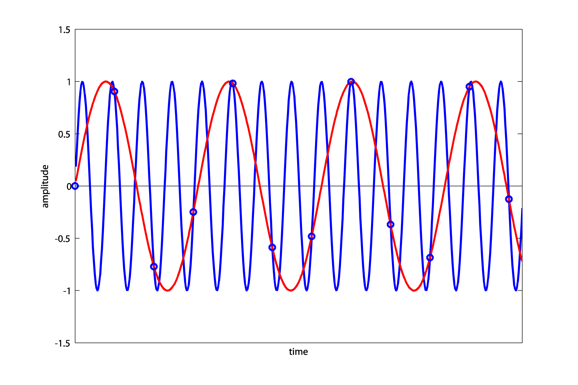
In the first case, when the actual frequency is less than or equal to the Nyquist frequency, the sampling rate is sufficient and there is no aliasing. In the second case, when the actual frequency is between the Nyquist frequency and the sampling rate, the observed frequency is equal to the sampling rate minus the actual frequency. For example, a sampling rate of 1000 Hz causes an 880 Hz sound wave to alias to 120 Hz (Figure 5.35).
For an actual frequency that is above the sampling rate, like 1320 Hz, the calculations are as follows:
$$p=1320/500=2$$
$$r=1320\,mod\,500=320$$
p is even, so
$$f_{obs}=320$$
Thus, a 1320 Hz wave sampled at 1000 Hz aliases to 320 Hz (Figure 5.36).
For an actual frequency of 1760 Hz, we have
$$p=1760/500=3$$
$$r=1760\,mod\,500=260$$
p is odd, so
$$f_{obs}=500-260=240$$
Thus, a 1760 Hz wave sampled at 1000 Hz aliases to 240 Hz (Figure 5.37).

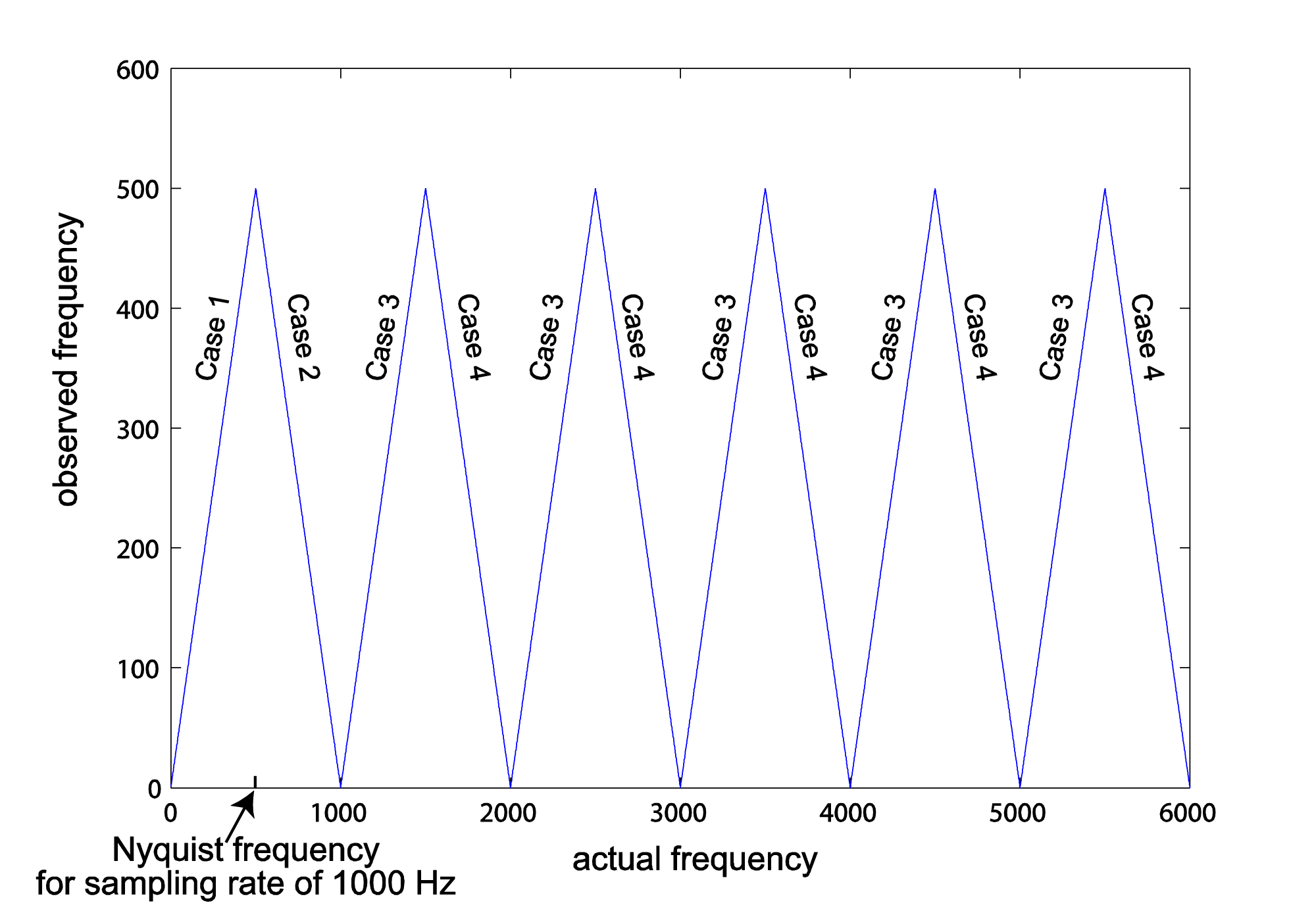
The graph in Figure 5.38 shows f_obs as a function of f_act for a fixed sampling rate, in this case 1000 Hz. For a different sampling rate, the graph would still have the same basic repeated-peak shape, but its peaks would be at different places. The first peak from the left is located at the Nyquist frequency on the horizontal axis, which is half the sampling rate. After the first peak, Case 3 is always on the left side of a peak and Case 4 is always on the right.
5.3.5 Simulating Sampling and Quantization in MATLAB
Now that you’ve looked more closely at the process of sampling and quantization in this chapter, you should have a clearer understanding of the MATLAB and C++ examples in Chapters 2 and 3.
[aside]An alternative way to get the points at which samples are taken is this:
f = 440;
sr = 44100;
s = 1;
t = [1:sr*s];
y = sin(2*pi*f*(t/sr*s));
Plugging in the numbers from this example, you get
y = sin(2*pi*440*t/44100);
[/aside]
In MATLAB, you can generate samples from a sine wave of frequency f at a sampling rate r for s seconds in the following way:
f = 440;
sr = 44100;
s = 1;
t = linspace(0,s,sr * s);
y = sin(2*pi*f*t);
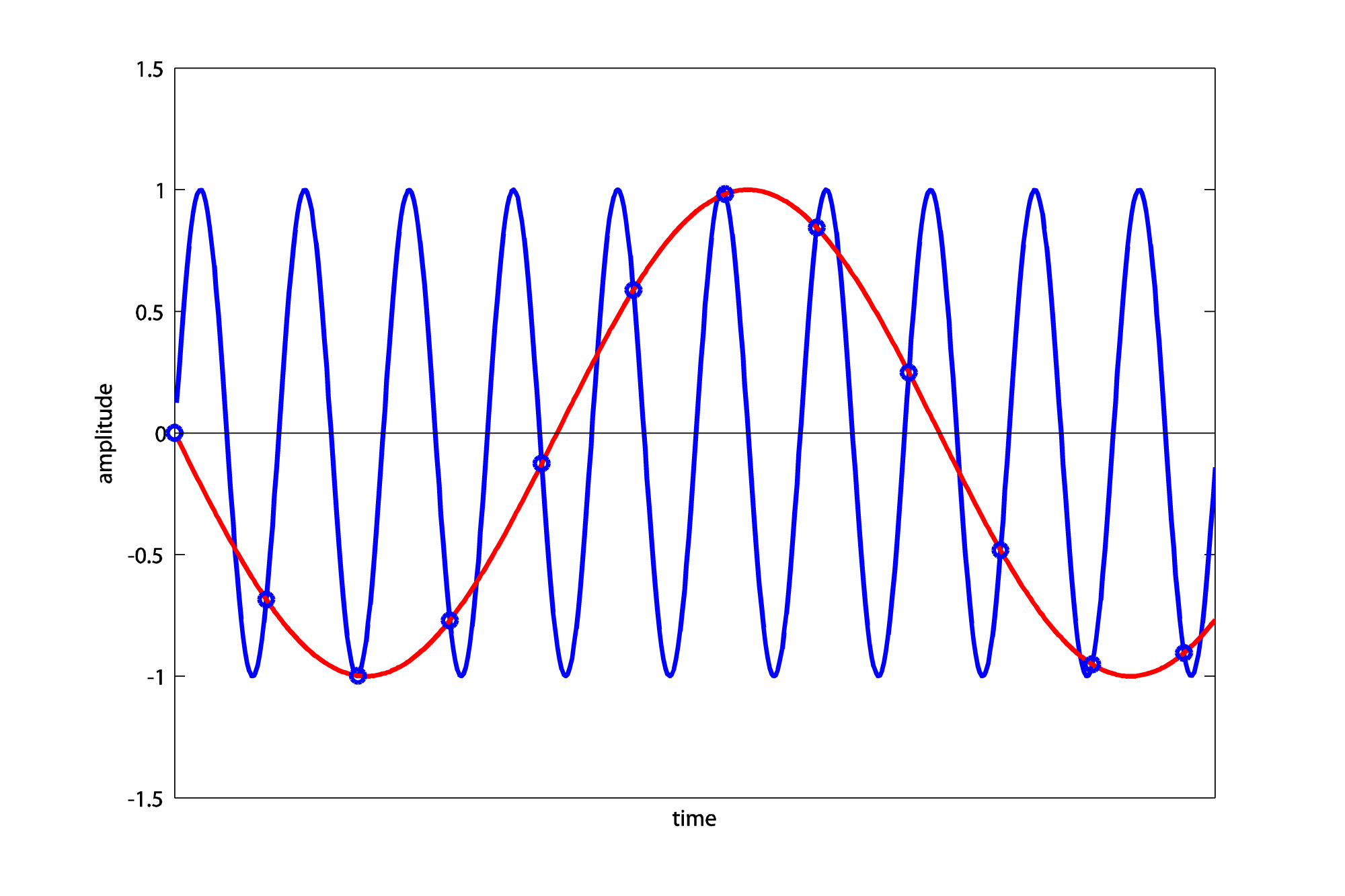
We’ve looked at statements like these in Chapter 2, but let’s review. The statement linspace(0, s, sr * s) creates a one-dimensional array (which can also be called a vector) of sr*s values evenly spaced between 0 and s. These are the points at which the samples are to be taken. One statement in MATLAB can cause an operation to be done on every element of a vector. For example, y = sin(2*pi*f*t) takes the sine on each element of t and stores the result in vector y. Since t has 44100 values in it, y does also. In this way, MATLAB simulates the sampling process for a single-frequency sound wave.
[wpfilebase tag=file id=63 tpl=supplement /]
Quantization can also be simulated in MATLAB. Notice that from the above sequence of commands, all the elements of y are between -1 and 1. To quantize these values to a bit depth of b, you can do the following:
b = 8;
sample_max = 2^(b-1)-1;
y_quantized = floor(y*sample_max);
The plot function graphs the result.
plot(t, y);
If we want to zoom in on the first, say, 500 values, we can do so with
plot(t(1:500), y(1:500));
With these basic commands, you can do the suggested exercise linked with this section, which has you experiment with quantization error and dynamic range at various bit depths.
5.3.6 Simulating Sampling and Quantization in C++
[wpfilebase tag=file id=93 tpl=supplement /]
[wpfilebase tag=file id=95 tpl=supplement /]
You can simulate sampling and quantization in C++ just as you can in MATLAB. The difference is that you need loops to operate on arrays in C++, while one command in MATLAB can cause an operation to be performed on each element in an array. (You can also write loops in MATLAB, but it isn’t necessary where array operations are available.) For example, the equivalent of the MATLAB lines above is given in C++ below. (We use mostly C syntax but, for simplicity, include some C++ features like dynamic allocation with new and the ability to declare variables anywhere in the program.)
int f = 440;
int r = 44100;
double s = 1;
int b = 8;
double* y = new double[r*s];
for (int t = 0; t < r * s; t++)
	y[t] = sin(2*PI*f*(t/(r*s)));
To quantize the samples in y to a bit depth of b, we do this:
int sample_max = pow(2, b-1) – 1;
short* y_quantized = new short[r*s];
for (int i = 0; i < r * s; i++)
	y_quantized[i] = floor(y * sample_max);
The suggested programming exercise linked with this section uses code such as this to implement Algorithm 5.1 for aliasing and to experiment with quantization error at various bit depths.
[separator top=”0″ bottom=”1″ style=”none”]
5.3.7 The Mathematics of Dithering and Noise Shaping
[wpfilebase tag=file id=97 tpl=supplement /]
[wpfilebase tag=file id=61 tpl=supplement /]
Dithering is described in Section 5.1.2.5 as the addition of low-amplitude random noise to an audio signal as it is being quantized. The purpose of dithering is to prevent neighboring sample values from quantizing all to the same level, which can cause breaks or choppiness in the sound. Noise shaping can be performed in conjunction with dithering to raise the noise to a higher frequency where it is not noticed as much. Now let’s look at the mathematics of dithering and noise shaping.
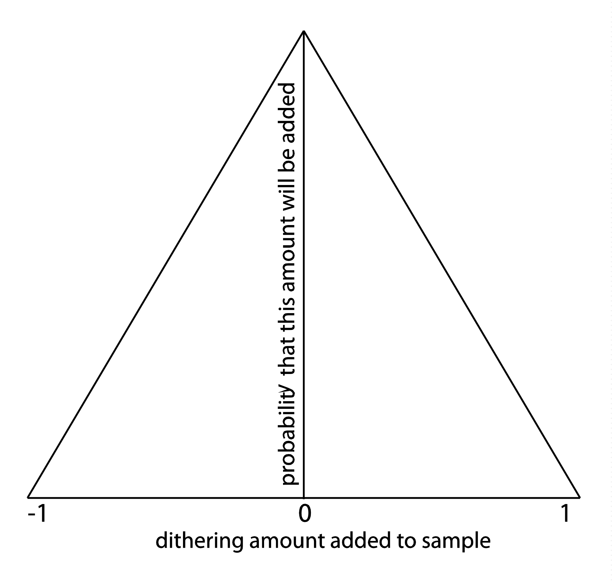
First, the amount of random noise to be added to each sample must be determined. A probability density function can be used for this purpose. We’ll use the triangular probability density function graphed in Figure 5.39 as an example. This graph depicts the following:
- There is 0 probability that an amount less than -1 and greater than 1 will be added to any given sample.
- As x moves from -1 to 0 and as x moves from 1 to 0, there is an increasing probability that x will be added to any given sample.
Thus, it’s most likely that some number close to 0 will be added as dither, and the highest magnitude value to be added or subtracted is 1. If you were to implement dithering yourself in MATLAB or a C++ program (as in the exercises associated with this section), you could create a triangular probability density function by getting a random number between -1 and 0 and another between 0 and 1 and summing them.
Audio processing programs like Adobe Audition or Sound Forge offer a variety of probability functions for noise shaping, as shown in Figure 5.40. The rectangular probability density function gives equal probability for all numbers within a given range. The Gaussian function weighs the probabilities according to a Gaussian rather than a triangular shape, so it would look like Figure 5.39 except more bell-shaped. This creates noise that is more like common environmental noise, like tape hiss.

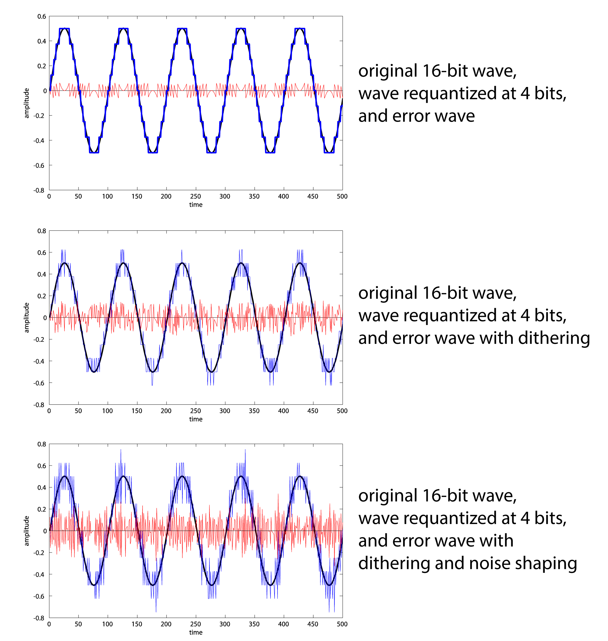
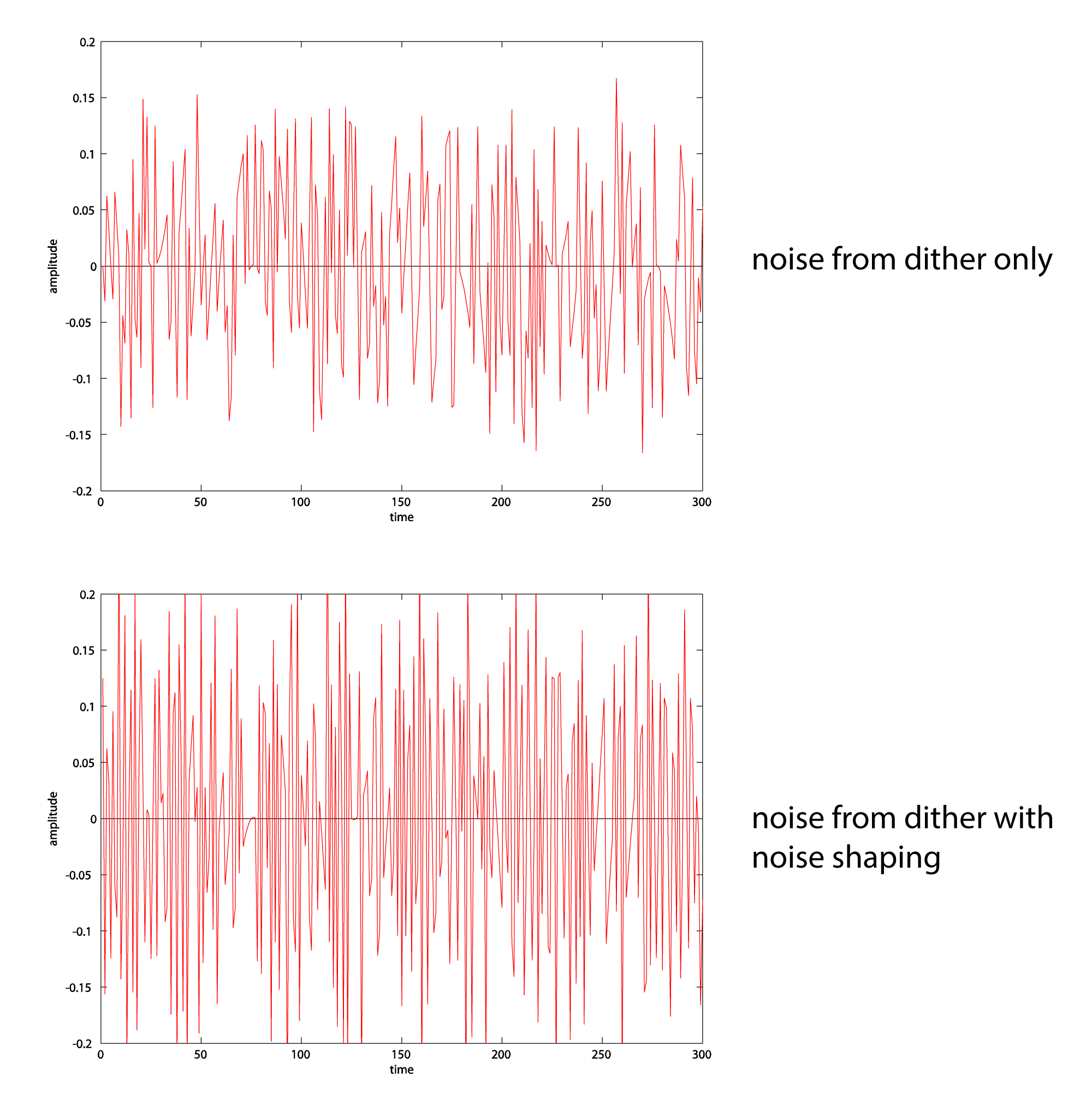
Requantization without dithering, with dithering, and with dithering and noise shaping are compared in Figure 5.41. A 16-bit audio file has been requantized to 4 bits (an unlikely scenario, but it makes the point). From these graphs, it may look like noise shaping adds additional noise. In fact, the reason the noise graph looks more dense when noise shaping is added is that the frequency components are higher.
To examine this more closely, we can extract the noise into a separate audio file by subtracting the original file from the requantized one. We’ve done this for both cases – noise from dither, and noise from dither and noise shaping. (The noise includes the quantization error.) Closeups of the noise graphs are shown in Figure 5.42. What you should notice is that dither-with-noise-shaping noise has higher frequency components than dither-only noise.
You can see this also in the spectral view of the noise files in Figure 5.43. In a spectral view of an audio file, time is on the x-axis, frequency is on the y-axis, and the amplitude of the frequency is represented by the color at each (x,y) point. The lowest amplitude is represented by blue, medium amplitudes move from red to orange, and the highest amplitudes move from yellow to white. You can see that when dithering alone is applied, the noise is spread out over all frequencies. When noise shaping is added to dithering, there is less noise at low frequency and more noise at high frequency. The effect is to pull more of the noise to high frequencies, where it is noticed less by human ears. (ADCs also can filter out the high frequency noise if it is above the Nyquist frequency.)

Noise shaping algorithms, first developed by Cutler in the 1950s, operate by computing the error from quantizing a sample (including the error from dithering and noise shaping) and adding this error to the next sample before it is quantized. If the error from the ith sample is positive, then, by subtracting the error from the next sample, noise shaping makes it more likely that the error for the i+1st sample will be negative. This causes the error wave to go up and down more frequently; i.e., the frequency of the error wave is increased. The algorithm is given in Algorithm 5.2. You can output your files as uncompressed RAW files, import the data into MATLAB, and graph the error waves, comparing the shape of the error with dither-only and with noise shaping using various values for c, the scaling factor. The algorithm given is the most basic kind of noise shaping you can do. Many refinements and variations of this algorithm have been implemented and distributed commercially.
[equation class=”algorithm” caption=”Algorithm 5.2″]
algorithm noise_shape {
/*Input:
     b_orig, the original bit depth
     b_new, the new bit depth to which samples are to be quantized
     F_in, an array of N digital audio samples that are to be
     quantized, dithered, and noise shaped.  It’s assumed that these are read
     in from a RAW file and are values between
     –2^b_orig-1 and (2^b_orig-1)-1.
     c, a scaling factor for the noise shaping
Output:
     F_out, an array of N digital audio samples quantized to bit
     depth b_new using dither and noise shaping*/

   s = (2^b_orig)/(2^b_new);
   c = 0.8;  //Other scaling factors can be tried.*/
   e = 0;
   for (i = 0; i < N; i++) {
/*Get a random number between −1 and 1 from some probability density function*/
      d = pdf();
      F_scaled  = F_in[i] / s;  //Integer division, discarding remainder
      F_scaled_plus_dith_and_error = F_scaled + d + c*e;
      F_out[i] =  floor(F_scaled_plus_dith_and_error);
      e = F_scaled – F_out[i];
   }
}
[/equation]
5.3.8 Algorithms for Audio Companding and Compression
5.3.8.1 Mu-law Encoding
Mu-law encoding (also denoted μ-law) is a nonlinear companding method used in telecommunications. Companding is a method of compressing a digital signal by reducing the bit depth before it is transmitted and then expanding it when it is received. The advantage of mu-law encoding is that it preserves some of the dynamic range that would be lost if a linear method of reducing the bit depth were used instead. Let’s look more closely at the difference between linear and nonlinear methods of bit depth reduction.
Picture this scenario. A telephone audio signal is to be transmitted. It is originally 16 bits. To reduce the amount of data that has to be transmitted, the audio data is reduced to 8 bits. In a linear method of bit depth reduction, the amount of quantization error possible at low amplitudes is the same as the amount of error possible at high amplitudes. However, this means that the ratio of the error to the sample value is greater for low amplitude samples than for high. Let’s assume that in converting from 16 bits to 8 bits is done by dividing by the sample value by 256 and rounding down. Consider a 16-bit sample that is originally 32767, the highest positive value possible. (16-bit samples range from -32768 to 32767.) Converted to 8 bits, the sample value becomes 127. (32767/256 = 127 with a remainder of 255.) The error from rounding is 255/32768. This is an error of less than 1%. But compare this to the error for the lowest magnitude 16-bit samples, those between 0 and 255. They all round to 0 when reduced to a bit depth of 8, which is 100% error. The point is that with a linear bit depth reduction method, rounding down has a greater impact on low amplitude samples than on high amplitude ones.
In a nonlinear method such as mu-law encoding, when the bit depth is reduced, the effect is that not all samples are encoded in the same number of bits. Low amplitude samples are given more bits to protect them from quantization error.
Equation 5.5 (which is, more precisely, a function) effectively redistributes the sample values so that there are more quantization levels at lower amplitudes and fewer quantization levels at higher amplitudes. For requantization from 16 to 8 bits, μ = 255.
[equation caption=”Equation 5.5″]
Let x be a sample value, $$-1\leq x\leq 1$$. Let $$sign\left ( x \right )=-1$$ if x is negative and $$sign\left ( x \right )=1$$ otherwise.
Then the mu-law function (also denoted μ-law) is defined by
$$!mu\left ( x \right )=sign\left ( x \right )\left ( \frac{ln\left ( 1+\mu \left | x \right | \right )}{ln\left ( 1+\mu \right )} \right )=sign\left ( x \right )\left ( \frac{ln\left ( 1+255\left | x \right | \right )}{5.5452} \right )\:for\: \mu =255$$
[/equation]
[wpfilebase tag=file id=65 tpl=supplement /]
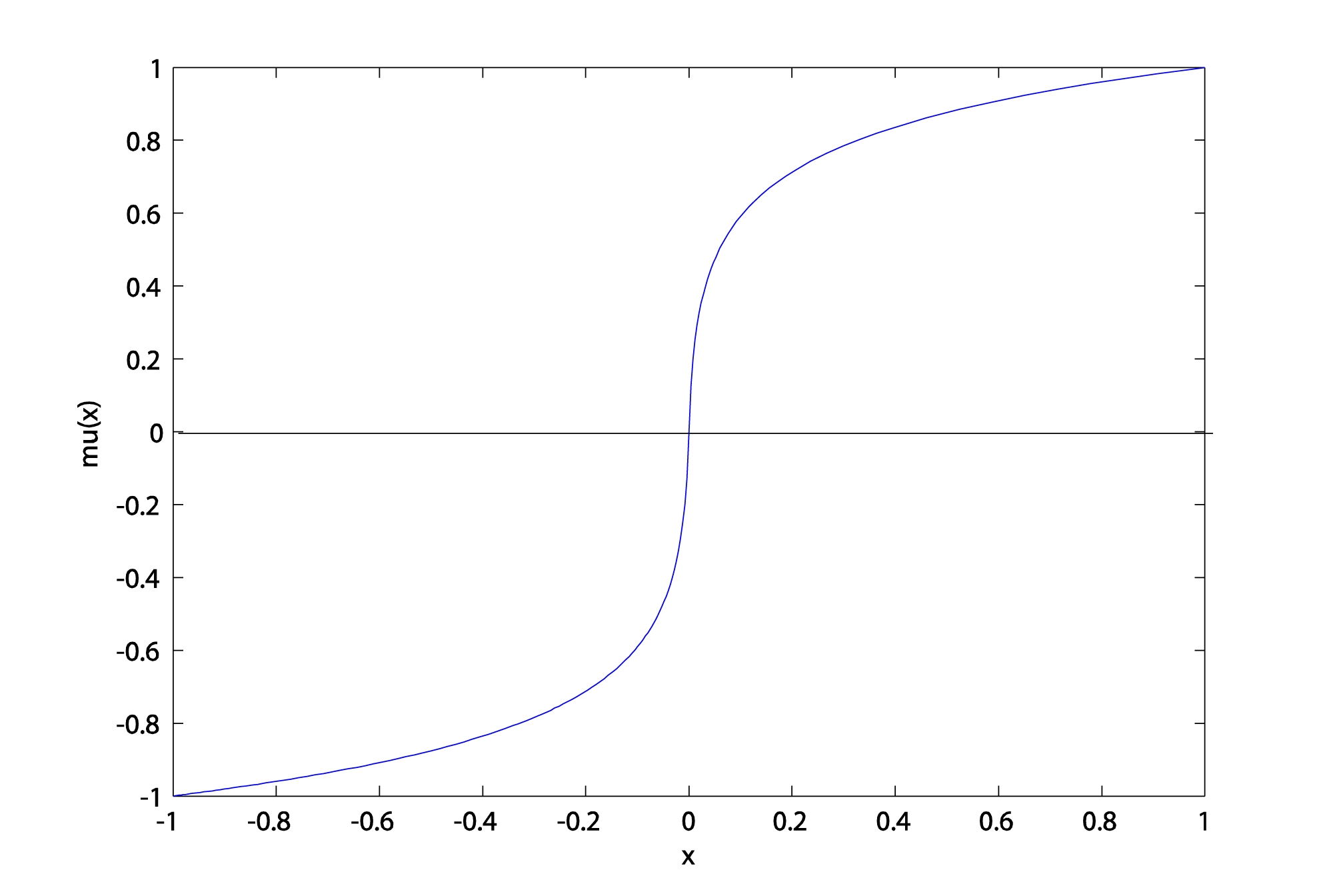
The graph of the mu-law function in Figure 5.44 has the original sample value (on a scale of -1 to 1) on the x-axis and the sample value after it is run through the mu-law function on the y-axis. Notice that the difference between, say, mu(0.001) and mu(0.002) is greater than the difference between mu(0.981) and mu(0.982).
mu(0.001) = 0.0410
mu(0.002) = 0.0743
mu(0.981) = 0.9966
mu(0.982) = 0.9967
The mu-law function has the effect of “spreading out” the quantization intervals more at lower amplitudes.
[wpfilebase tag=file id=99 tpl=supplement /]
It may be easier to see how this works if we start with sample values on a 16-bit scale (i.e., between -32768 and 32767) and then scale the results of the mu-law function back to 8 bits. For example, what happens if we begin with sample values of 33, 66, 32145, and 32178? (Notice that these normalize to 0.001, 0.002, 0.981, and 0.982, respectively, on a -1 to 1 scale.)
mu(33/32768) = 0.0412;
floor(128*0.0412) = 5;
mu(66/32768) = 0.0747;
floor(128* 0.0747) = 9;
mu(32145/32768) = 0.9966;
floor(128*0.9966) = 127;
mu(32178/32768) = 0.9967;
floor(128*0.9967) = 127;
The sample values 33 and 66 on a 16-bit scale become 5 and 9, respectively, on an 8-bit scale. The sample values 32145 and 32178 both become 127 on an 8-bit scale. Even though the difference between 66 and 33 is the same as the difference between 32178 and 32145, 66 and 33 fall to different quantization levels when they are converted to 8 bits, but 32178 and 32145 fall to the same quantization level. There are more quantization levels at lower amplitudes after themu-law function is applied.
The result is that there is less error at low amplitudes, after requantization to 16 bits, than there would have been if a linear quantization method had been used. Equation 5.6 shows the function for expanding back to the original bit depth.
[equation caption=”Equation 5.6″]
Let x be a μ-law encoded sample value, $$-1\leq x\leq 1$$. Let $$sign\left ( x \right )=-1$$ if x is negative and $$sign\left ( x \right )=1$$ otherwise.
Then the inverse μ-law function is defined by
$$!\left ( \mu\, inverse\left ( x \right )=sign\left ( x \right )\, \left ( \frac{\left ( \mu +1 \right )^{\left | x \right |}-1}{\mu } \right )=sign\left ( x \right )\left ( \frac{256^{\left | x \right |}-1}{255} \right )\, for\: \mu =255 \right )$$
[/equation]
Our original 16-bit values of 33 and 66 convert to 5 and 9, respectively, in 8 bits. We can convert them back to 16 bits using the inverse mu-law function as follows:
mu_inverse(5/128) = .00094846
ceil(32768* .00094846) = 32
mu_inverse(9/128) = 0.0019
ceil(32768*0.0019) = 63
The original value of 33 converted back to 32. The original value of 66 converted back to 63. On the other hand, look what happens to the higher amplitude values that were originally 32145 and 32178 and converted to 127 at 8 bits.
mu_inverse(127/128) = 0.9574
ceil(32768*0.9574) = 31373
Both 32145 and 32178 convert back to 31373.
With mu-law encoding, the results are better than they would have been if a linear method of bit reduction had been used. Let’s look at the linear method. Again suppose we convert from 16 to 8 bits by dividing by 256 and rounding down. Then both 16-bit values of 33 and 66 would convert to 0 at 8 bits. To convert back up to 16 bits, we multiply by 256 again and still have 0. We’ve lost all the information in these samples. On the other hand, by a linear method both 32145 and 32178 convert to 125 at 8 bits. When they’re scaled back to 16 bits, they both become 32000. A comparison of percentage errors for all of these samples using the two conversion methods is shown in Table 5.2. You can see that mu-law encoding preserves information at low amplitudes that would have been lost by a linear method. The overall result is that with a bit depth of only 8 bits for transmitting the data, it is possible to retrieve a dynamic range of about 12 bits or 72 dB when the data is uncompressed to 16 bits (as opposed to the 48 dB expected from just 8 bits). The dynamic range is increased because fewer of the low amplitude samples fall below the noise floor.
[table caption=”Table 5.2 Comparison of error in linear and nonlinear compounding” width=”80%”]
original sample~~at 16 bits,”sample after linear~~companding,~~16 to 8 to 16″,error,”sample after nonlinear~~companding,~~16 to 8 to 16″,percentage~~error
33,0,100%,32,3%
66,0,100%,63,4.50%
32145,32000,0.45%,31373,2.40%
32178,32000,0.55%,31373,2.50%
[/table]
Rather than applying the mu-law function directly, common implementations of mu-law encoding achieve an equivalent effect by dividing the 8-bit encoded sample into a sign bit, mantissa, and exponent, similar to the way floating point numbers are represented. An advantage of this implementation is that it can be performed with fast bit-shifting operations. The programming exercise associated with this section gives more information about this implementation, comparing it with a literal implementation of the mu-law and inverse mu-law functions based on logarithms.
Mu-law encoding (and its relative, A-law, which is used Europe) reduces the amount of data in an audio signal by quantizing low-amplitude signals with more precision than high amplitude ones. However, since this bit-depth reduction happens in conjunction with digitization, it might more properly be considered a conversion rather than a compression method.
Actual audio compression relies on an analysis of the frequency components of the audio signal coupled with a knowledge of how the human auditory system perceives sound – a field of study called psychoacoustics. Compression algorithms based on psychoacoustical models are grouped under the general category of perceptual encoding, as is explained in the following section.
5.3.8.2 Psychoacoustics and Perceptual Encoding
Psychoacoustics is the study of how the human ears and brain perceive sound. Psychoacoustical experiments have shown that human hearing is nonlinear in a number of ways, including perception of octaves, perception of loudness, and frequency resolution.
For a note C2 that is one octave higher than a note C1, the frequency of C2 is twice the frequency of C1. This implies that the frequency width of a lower octave is smaller than the frequency width of a higher octave. For example, the octave C5 to C6 is twice the width of C4 to C5. However, the octaves are perceived as being the same width in human hearing. In this sense, our perception of octaves is nonlinear.
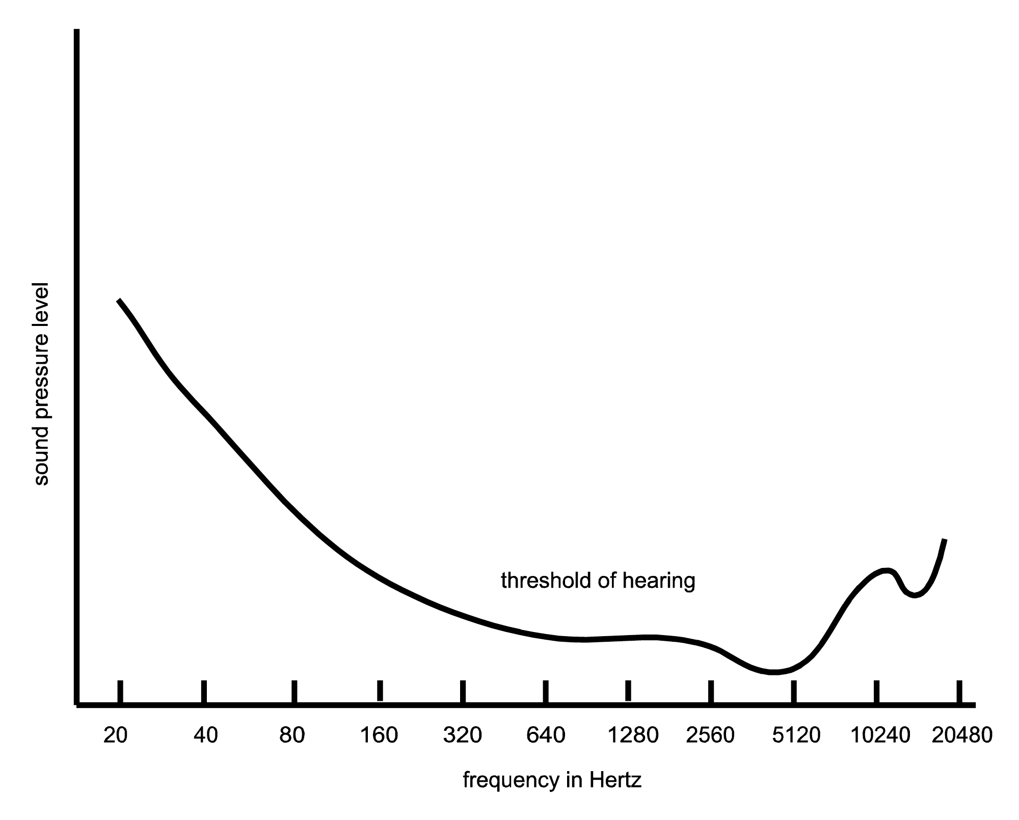
Humans hear best (i.e., have the most sensitivity to amplitude) in the range of about 1000 to 5000 Hz, which is close to the range of the human voice. We hear less well at both ends of the frequency spectrum. This is illustrated in Figure 5.45, which shows the shape of the threshold of hearing plotted across frequencies.
Human ability to distinguish between frequencies decreases nonlinearly from low to high frequencies. At the very lowest audible frequencies, we can tell the difference between pitches that are only a few Hz apart, while at high frequencies the pitches must be separated by more than 100 Hz before we notice a difference. This difference in frequency sensitivity arises from the fact that the inner ear is divided into critical bands. Each band is tuned to a range of frequencies. Critical bands for low frequencies are narrower than those for high ones. Between frequencies of 1 and 500 Hz, critical bands have a width of about 100 Hz or less, whereas the width of the critical band at the highest audible frequency is about 4000 Hz.
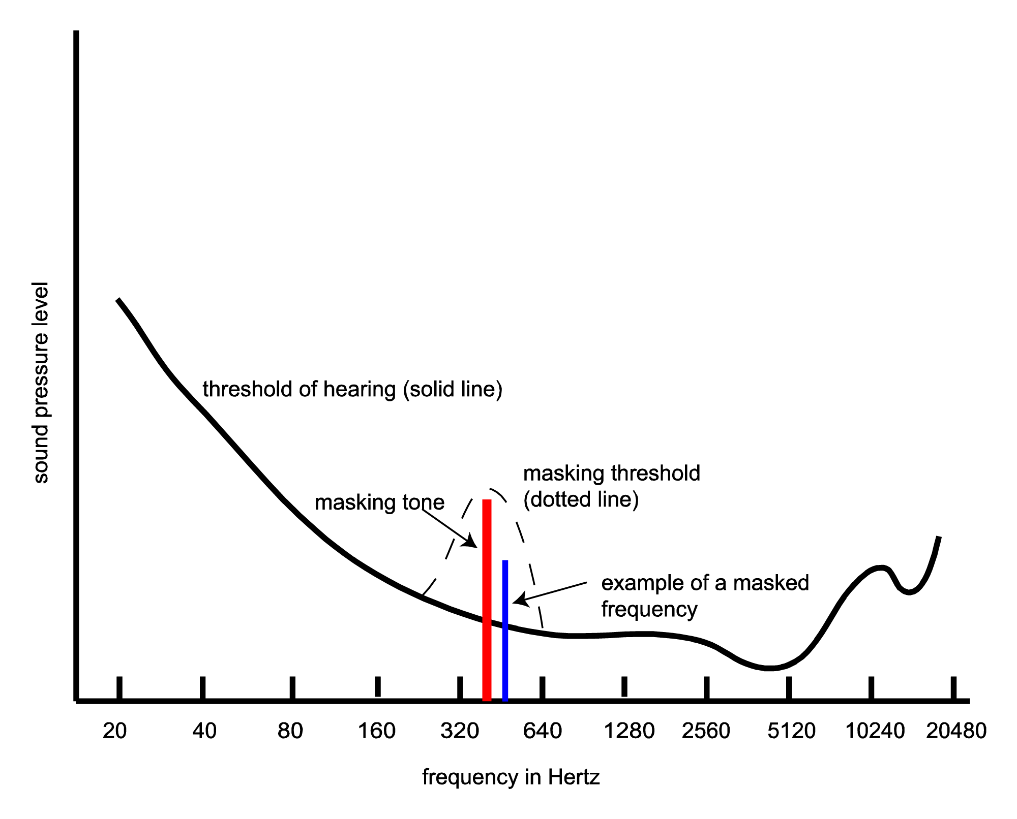
The goal of applying psychoacoustics to compression methods is to determine the components of sounds that human ears don’t perceive very well, if at all. These are the parts that can be discarded, thereby decreasing the amount of data that must be stored in digitized sound. An understanding of critical bands within the human ear helps in this regard. Within a band, a phenomenon called masking can occur. Masking results when two frequencies are received by a critical band at about the same moment in time, one of the frequencies being significantly louder than the first such that it makes the first inaudible. The loud frequency is called the masking tone, and the quiet one is the masked frequency. Masking causes the threshold of hearing to be raised within a critical band in the presence of a masking tone. The new threshold of hearing is called the masking threshold, as depicted in Figure 5.46. Note that this graph represents the masking tone in one critical band in a narrow window of time. Audio compression algorithms look for places where masking occurs in all of the critical bands over each consecutive window of time for the duration of the audio signal.
Another type of masking, called temporal masking, occurs with regard to transients. Transients are sudden bursts of sounds like drum beats, hand claps, finger snaps, and consonant sounds. When two transients occur close together in time, the louder one can mask the weaker one. Identifying instances of temporal masking is another important part of perceptual encoding.
5.3.8.3 MP3 and AAC Compression
[aside]MPEG is an acronym for Motion Picture Experts Group and refers to a family of compression methods for digital audio and video. MPEG standards were developed in phases and layers beginning in 1988, as outlined in Table 5.3. The phases are indicated by Arabic numerals and the layers by Roman numerals.[/aside]
Two of the best known compression methods that use perceptual encoding are MP3 and AAC. MP3 is actually a shortened name for MPEG-1 Audio Layer III. It was developed through a collaboration of scientists at Fraunhofer IIS, AT&T Bell Labs, Thomason-Brandt, CCETT, and others and was approved by ISO/IEC as part of the MPEG standard in 1991. MP3 was a landmark compression method in the way that it popularized the exchange of music by means of the web. Although MP3 is a lossy compression method in that it discards information that cannot be retrieved, music lovers were quick to accept the tradeoff between some loss of audio quality and the ability to store and exchange large numbers of music files.
AAC (Advanced Audio Coding) is the successor of MP3 compression, using similar perceptual encoding techniques but improving on these and supporting more channels, sampling rates, and bit rates. AAC is available within both the MPEG-2 and MPEG-4 standards and is the default audio compression method for iPhones, iPods, iPads, Android phones, and a variety of video game consoles. Table 5.1 shows the filename extensions associated with MP3 and AAC compression.
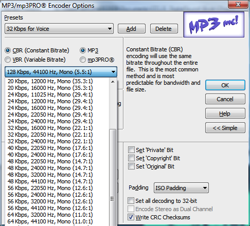
You may have read that MP3 offers a compression ratio of about 11 to 1. This number gives you a general idea, but exact compression ratios vary. Table 5.3 shows ranges of bit rates available for different layers within the MPEG standard. Typically, an MP3 compressor offers a number of choices of bit rates, these varying with sampling rates, as shown in Figure 5.47 for Adobe Audition’s MP3/mp3Pro encoder. The bit rate indicates how many bits of compressed data is generated per second. A constant bit rate of 128 kb/s for mono audio sampled at 44100 Hz with 16 bits per sample gives a compression ratio of 5.5:1, as shown in the calculation below.
44100 samples/s * 16 = 705600 b/s uncompressed
705600 uncompressed : 128000 b/s compressed ≈ 5.5:1
For stereo (32 bits per sample) at a sampling rate of 44100, compressed to 128 kb/s, the compression ratio is approximately 11:1. This is where the commonly-cited compression ratio comes from – the fact that frequently, MP3 compression is used on CD quality stereo at a bit rate of 128 kb/s, which most listeners seem to think gives acceptable quality. For a given implementation of MP3 compression and a fixed sampling rate, bit depth, and number of channels, a higher bit rate yields better quality in the compressed audio than a lower bit rate. When fewer bits are produced per second of audio, more information must be thrown out.
[table caption=”Table 5.3 MPEG audio” width=”80%”]
Version,Bit rates*,Applications,Channels,Sampling rates supported
MPEG-1,,”CD, DAT, ISDN, video games, digital audio broadcasting, music shared on the web, portable music players”,mono or stereo,”32, 44.1, and 48 kHz”
Layer I,32_448 kb/s,,,”(and 16, 22.05, and 24 kHz for MPEG-2 LSF, low sampling frequency)”
Layer II,32_384 kb/s,,,
Layer III,32_320 kb/s,,,
MPEG-2 ,,”multichannels, multilingual extensions”,5.1 surround,”32, 44.1, and 48 kHz ”
Layer I,32_448 kb/s,,,
Layer II,32_384 kb/s,,,
Layer III,32_320 kb/s,,,
AAC in MPEG-2 and MPEG-4 (Advanced Audio Coding),8 _384 kb/s,”multichannels, music shared on the web, portable music players, cell phones”,up to 48 channels,”32, 44.1, and 48 kHz and other rates between 8 and 96 kHz”
*Available bit rates vary with sampling rate.,,,,
[/table]
The MPEG standard does not prescribe how compression is to be implemented. Instead, it prescribes the format of the encoded audio signal, which is a bit stream made up of frames with certain headers and data fields. The MPEG standard suggests two psychoacoustical models that could accomplish the encoding, the second model, used for MP3, being more complex and generally resulting in greater compression than the first. In reality, there can be great variability in the time efficiency and quality of MP3 encoders. The advantage to not dictating details of the compression algorithm is that implementers can compete with novel implementations and refinements. If the format of the bit stream is always the same, including what each part of the bit stream represents, then decoders can be implemented without having to know the details of the encoder’s implementation.
An MP3 bit stream is divided into frames each of which represents the compression of 1152 samples. The size of the frame containing the compressed data is determined by the bit rate, a user option that is set prior to compression. As before, let’s assume that a bit rate of 128 kb/s is chosen to compress an audio signal with a sampling rate of 44.1 kHz. This implies that the number of frames of compressed data that must be produced per second is 44100/1152 ≈ 38.28. The chosen bit rate of 128 kb/s is equal to 16000 bytes per second. Thus, the number of bytes allowed for each frame is 16000/38.28 ≈ 418. You can see that if you vary the sampling rate or the bit rate, there will be a different number of bytes in each frame. This computation considers only the data part of each compressed frame. Actually, each frame consists of a 32-byte header followed by the appropriate number of data bytes, for a total of approximately 450 bytes in this example.
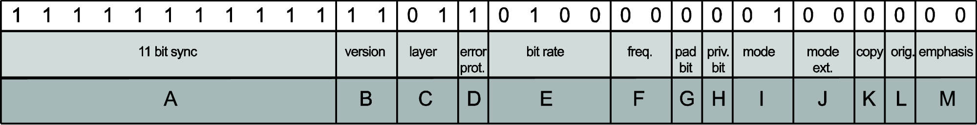
The format of the header is shown in Figure 5.48 and explained in Table 5.4.
[table caption=”Table 5.4 Contents of MP3 frame header” width=”80%”]
Field,Length in Bits,Contents
A,11,all 1s to indicate start of frame
B,2,MPEG-1 indicated by bits 1 1
C,2,Layer III indicated by bits 0 1
D,1,0 means protected by CRC* (with 16 bit CRC following header)
,,1 means not protected
E,4,bit rate index
,,0000 free
,,0001 32 kb/s
,,0010 40 kb/s
,,0011 48 kb/s
,,0100 56 kb/s
,,0101 64 kb/s
,,0110 80 kb/s
,,0111 96 kb/s
,,1000 112 kb/s
,,1001 128 kb/s
,,1010 160 kb/s
,,1011 192 kb/s
,,1100 224 kb/s
,,1101 256 kb/s
,,1110 320 kb/s
,,1111 bad
F,2,frequency index
,,00 44100 Hz
,,01 48000 Hz
,,10 32000 Hz
,,11 reserved
G,1,0 frame is not padded
,,1 frame is padded with an extra byte
,,”Padding is used so that bit rates are fitted exactly to frames. For example, a 44100 Hz audio signal at 128 kb/s yields a frame of about 417.97 bytes”
H,1,”private bit, used as desired by implementer”
I,2,channel mode
,,00 stereo
,,01 joint stereo
,,10 2 independent mono channels
,,11 1 mono channel
J,2,mode extension used with joint stereo mode
K,1,0 if not copyrighted
,,1 if copyrighted
L,1,0 if copy of original media
,,1 if not
M,2,indicates emphasized frequencies
“*CRC stands for cyclical redundancy check, an error correcting code that checks for errors in the transmission of data.”[attr colspan=”3”]
[/table]
MP3 supports both constant bit rate (CBR) and variable bit rate (VBR). VBR makes it possible to vary the bit rate frame-by-frame, allocating more bits to frames that require greater frequency resolution because of the complexity of the sound in that part of the audio. This can be implemented by allowing the user to specify the maximum bit rate. An alternative is to allow the user to specify an average bit rate. Then the bit rate can vary frame-by-frame but is controlled so that it averages to the chosen rate.
A certain amount of variability is possible even within CBR. This is done by means of a bit reservoir in frames. A bit reservoir is a created from bits that do not have to be used in a frame because the audio being encoded is relatively simple. The reservoir provides extra space in a subsequent frame that may be more complicated and requires more bits for encoding.
Field I in Table 5.4 makes reference to the channel mode. MP3 allows for one mono channel, two independent mono channels, two stereo channels, and joint stereo mode. Joint stereo mode takes advantage of the fact that human hearing is less sensitive to the location of sounds that are the lowest and highest ends of the audible frequency ranges. In a stereo audio signal, low or high frequencies can be combined into a single mono channel without much perceptible difference to the listener. The joint stereo option can be specified by the user.
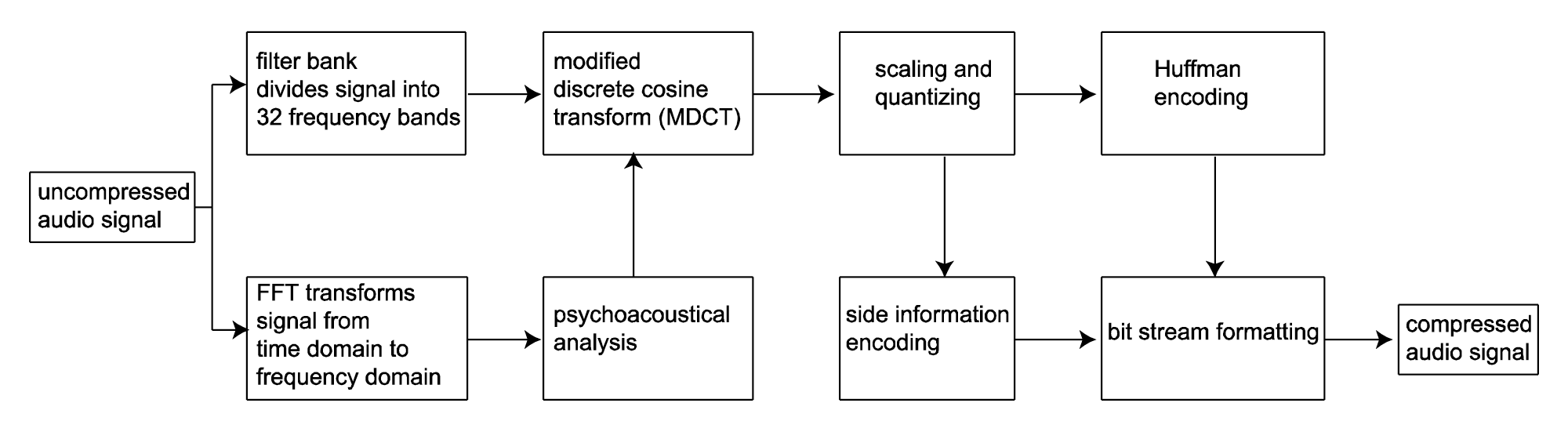
A sketch of the steps in MP3 compression is given in Algorithm 5.3 and the algorithm is diagrammed in Figure 5.49. This algorithm glosses over details that can vary by implementation but gives the basic concepts of the compression method.
[equation class=”algorithm” caption=”Algorithm 5.3 MP3 Compression”]
algorithm MP3 {
/*Input:  An audio signal in the time domain
  Output:  The same audio signal, compressed
/*
Process the audio signal in frames
For each frame {
   Use the Fourier transform to transform the time domain data to the frequency domain, sending
      the results to the psychoacoustical analyzer {
         Based on masking tones and masked frequencies, determine the signal-to-masking noise
            ratios (SMR) in areas across the frequency spectrum
         Analyze the presence and interactions of transients
      }
   Divide the frame into 32 frequency bands
   For each frequency band {
      Use the modified discrete cosine transform (MDCT) to divide each of the 32 frequency bands
         into 18 subbands, for a total of 576 frequency subbands
      Sort the subbands into 22 groups, called scale factor bands, and based on the SMR, determine
         a scaling factor for each scale factor band
      Use nonuniform quantization combined with scaling factors to quantize
      Encode side information
      Use Huffman encoding on the resulting 576 quantized MDCT coefficients
      Put the encoded data into a properly formatted frame in the bit stream
   }
}
[/equation]
Let’s look at the steps in this algorithm more closely.
1. Divide the audio signal in frames.
MP3 compression processes the original audio signal in frames of 1152 samples. Each frame is split into two granules of 576 samples each. Frames are encoded in a number of bytes consistent with the bit rate set for the compression at hand. In the example described above (with sampling rate of 44.1 kHz and requested bit rate of 128 kb/s), 1152 samples are compressed into a frame of approximately 450 bytes – 418 bytes for data and 32 bytes for the header.
2. Use the Fourier transform to transform the time domain data to the frequency domain, sending the results to the psychoacoustical analyzer.
The fast Fourier transform changes the data to the frequency domain. The frequency domain data is then sent to a psychoacoustical analyzer. One purpose of this analysis is to identify masking tones and masked frequencies in a local neighborhood of frequencies over a small window of time. The psychoacoustical analyzer outputs a set of signal-to-mask ratios (SMRs) that can be used later in quantizing the data. The SMR is the ratio between the amplitude of a masking tone and the amplitude of the minimum masked frequency in the chosen vicinity. The compressor uses these values to choose scaling factors and quantization levels such that quantization error mostly falls below the masking threshold. Step 5 explains this process further.
Another purpose of the psychoacoustical analysis is to identify the presence of transients and temporal masking. When the MDCT is applied in a later step, transients have to be treated in smaller window sizes to achieve better time resolution in the encoding. If not, one transient sound can mask another that occurs close to it in time. Thus, in the presence of transients, windows are made one third their normal size in the MDCT.
3. Divide each frame into 32 frequency bands
Steps 2 and 3 are independent and actually could be done in parallel. Dividing the frame into frequency bands is done with filter banks. Each filter bank is a bandpass filter that allows only a range of frequencies to pass through. (Chapter 7 gives more details on bandpass filters.) The complete range of frequencies that can appear in the original signal is 0 to ½ the sampling rate, as we know from the Nyquist theorem. For example, if the sampling rate of the signal is 44.1 kHz, then the highest frequency that can be present in the signal is 22.05 kHz. Thus, the filter banks yield 32 frequency bands between 0 and 22.05 kHz, each of width 22050/32, or about 689 Hz.
The 32 resulting bands are still in the time domain. Note that dividing the audio signal into frequency bands increases the amount of data by a factor of 32 at this point. That is, there are 32 sets of 1152 time-domain samples, each holding just the frequencies in its band. (You can understand this better if you imagine that the audio signal is a piece of music that you decompose into 32 frequency bands. After the decomposition, you could play each band separately and hear the musical piece, but only those frequencies in the band. The segments would need to be longer than 1152 samples for you to hear any music, however, since 1152 samples at a sampling rate of 44.1 kHz is only 0.026 seconds of sound.)
4. Use the MDCT to divide each of the 32 frequency bands into 18 subbands for a total of 576 frequency subbands.
The MDCT, like the Fourier transform, can be used to change audio data from the time domain to the frequency domain. Its distinction is that it is applied on overlapping windows in order to minimize the appearance of spurious frequencies that occur because of discontinuities at window boundaries. (“Spurious frequencies” are frequencies that aren’t really in the audio, but that are yielded from the transform.) The overlap between successive MDCT windows varies depending on the information that the psychoacoustical analyzer provides about the nature of the audio in the frame and band. If there are transients involved, then the window size is shorter for greater temporal resolution. Otherwise, a larger window is used for greater frequency resolution.
5. Sort the subbands into 22 groups, called scale factor bands, and based on the SMR, determine a scaling factor for each scale factor band. Use nonuniform quantization combined with scaling factors to quantize.
Values are raised to the ¾ power before quantization. This yields nonuniform quantization, aimed at reducing quantization noise for lower amplitude signals, where it has a more harmful impact.
The psychoacoustical analyzer provides information that is the basis for sorting the subbands into scale factor bands. The scale factor bands cover several MDCT coefficients and more closely match the critical bands of the human ear. This is one of the ways in which MP3 is an improvement over MPEG-1 Layers 1 and 2.
All bands are quantized by dividing by the same value. However, the values in the scale factor bands can be scaled up or down based on their SMR. Bands that have a lower SMR are multiplied by larger scaling factors because the quantization error for these bands has less impact, falling below the masking threshold.
Consider this example. Say that an uncompressed band value is 20,000 and values from all bands are quantized by dividing by 128 and rounding down. Thus the quantized value would be 156. When the value is restored by multiplying by 128, it is 19,968, for an error of $$\frac{32}{20000}=0.0016$$. Now supposed the psychoacoustical analyzer reveals that this band requires less precision because of a strong masking tone. Thus, it determines that the band should be scaled by a factor of 0.1. Now we have $$floor\left ( \frac{20000\ast 0.1}{128} \right )=15$$. Restoring the original value we get $$15\ast 128=19200$$, for an error of $$\frac{800}{20000}=0.04$$.
An appropriate psychoacoustical analysis provides scaling factors that increase the quantization error where it doesn’t matter, in the presence of masking tones. Scale factor bands effectively allow less precision (i.e., fewer bits) to store values if the resulting quantization error falls below the audible level. This is one way to reduce the amount of data in the compressed signal.
6. Encode side information.
Side information is the information needed to decode the rest of the data, including where the main data begins, whether granule pairs can share scale factors, where scale factors and Huffman encodings begin, the Huffman table to use, the quantization step, and so forth.
7. Use Huffman encoding on the resulting 576 quantized MDCT coefficients.
The result of the MDCT is 576 coefficients representing the amplitudes of 576 frequency subbands. Huffman encoding is applied at this point to further compress the signal.
Huffman encoding is a compression method that assigns shorter codes to symbols that appear more often in the signal or file being encoded and longer codes for symbols that appear infrequently. Here’s a sketch of how it works. Imagine that you are encoding 88 notes from a piano keyboard. You can use 7 bits for each note. (Six bits would be too few, since with six bits you can represent only $$2^{6}=64$$ different notes.) In a particular music file, you have 100 instances of notes. The number of instances of each is recorded in the table below. Not all 88 notes are used, but this is not important to the example. (This is just a contrived example, so don’t try to make sense of it musically.)
[table width=”30%”]
Note,Instances of Note
C4,31
B4,20
F3,16
D4,11
G4,8
E4,5
A3,4
B3,3
F4,2
[/table]
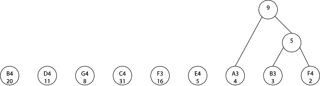
There are 100 notes to be encoded here. If each requires 7 bits, that’s 700 bits for the encoded file. It’s possible to reduce the size of this encoded file if we use fewer than 7 bits for the notes that appear most often. We can choose a different encoding by building what’s called a Huffman tree. We begin by creating a node (just a circle in a graph) for each of the notes in the file and the number of instances of that note, like this:
![]()
(The initial placement of the nodes isn’t important, although a good placement can make the tree look neater after you’ve finished joining nodes.) Now the idea is to combine the two nodes that have the smallest value, making a node above, marking it with the sum of the chosen nodes’ values, and joining the new node with lines to the nodes below. (The lines connecting the nodes are called arcs.) B3/3 and F4/2 have the smallest values, so we join them, like this:
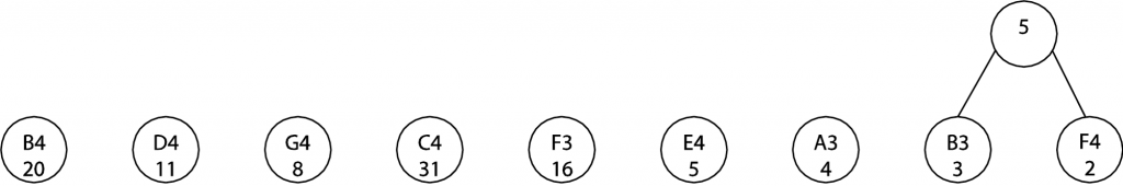
At the next step, A3/4 and the 5 node just created can be combined. (We could also combine A3/4 with E4/5. The choice between the two is arbitrary.) The sum of the instances is 9.
In the next two steps, we combine E4/5 with 9 and then D4 with G4, as shown.
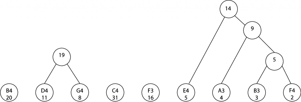
Continuing in this manner, the final tree becomes this:
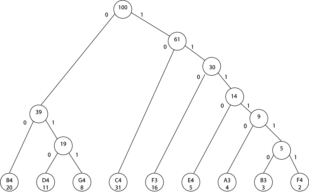
Notice that the left arc from each node has been labeled with a 0 and the right with a 1. The nodes at the bottom represent the notes to be encoded. You can get the code for a note by reading the 0s and 1s on the arcs that take you from the top node to one of the notes at the bottom. For example, to get to B4, you follow the arcs labeled 0 0. Thus, the new encoding for B4 is 0 0, which requires only two bits. To get to B3, you follow the arcs labeled 1 1 1 1 1 0. The new encoding for B3 is 1 1 1 1 1 0, which requires six bits. All the new encodings are given in the table below:
[table width=”50%”]
Note,Instances of Note,Code in Binary,Number of Bits
C4,31,10,2
B4,20,0,2
F3,16,110,3
D4,11,10,3
G4,8,11,3
E4,5,1110,4
A3,4,11110,5
B3,3,111110,6
F4,2,111111,6
[/table]
Note that not all notes are encoded in the same number of bits. This is not a problem to the decoder because no code is a prefix of any other. (This way, the decoder can figure out where a code ends without knowing its length.) With the encoding that we just derived, which uses fewer bits for notes that occur frequently, we need only 31*2 + 20*2 + 16*3 + 11*3 + 8*3 + 5*4 + 4*5 + 3*6 + 2*6 = 277 bits as opposed to the 700 needed previously.
This illustrates the basic concept of Huffman encoding. However, it is realized in a different manner in the context of MP3 compression. Rather than generate a Huffman table based on the data in a frame, MP3 uses a number of predefined Huffman tables defined in the MPEG standard. A variable in the header of each frame indicates which of these tables is to be used.
Steps 5, 6, and 7 can be done iteratively. After an iteration, the compressor checks that the noise level is acceptable and that the proper bit rate has been maintained. If there are more bits that could be used, the quantizer can be reduced. If the bit limit has been exceeded, quantization must be done more coarsely. The level of distortion in each band is also analyzed. If the distortion is not below the masking threshold, then the scale factor for the band can be adjusted.
8. Put the encoded data into a properly formatted frame in the bit stream.
The header of each frame is as shown in Table 5.4. The data part of each frame consists of the scaled, quantized MDCT values.
AAC compression, the successor to MP3, uses similar encoding techniques but improves on MP3 by offering more sampling rates (8 to 96 kHz), more channels (up to 48), and arbitrary bit rates. Filtering is done solely with the MDCT, with improved frequency resolution for signals without transients and improved time resolution for signals with transients. Frequencies over 16 kHz are better preserved. The overall result is that many listeners find AAC files to have better sound quality than MP3 for files compressed at the same bit rate.
5.3.8.4 Lossless Audio Compression
Lossless audio codecs include FLAC, Apple Lossless, MPEG-4 ALS, and Windows Media Audio Lossless, among others. All of these codecs compress audio in a way that retains all the original information. The audio, upon decompression, is identical to the original signal (disregarding insignificant computation precision errors). Lossless compression generally reduces an audio signal to about half its original size. Let’s look at FLAC as an example of how it’s done.
Like a number of other lossless codecs, FLAC is based on linear predictive coding. The main idea is as follows:
- Consider the audio signal in the time domain.
- Come up with a function that reasonably predicts what an audio sample is likely to be based on the values of previous samples.
- Using that formula on n successive samples, calculate what n+1 “should” be. This value is called the approximation.
- Subtract the approximation from the actual value. The result is called the residual (or residue or error, depending on your source).
- Save the residual rather than the actual value in the compressed signal. Since the residual is likely to be less than the actual value, this saves space.
- The decoder knows the formula that was used for approximating a sample based on previous samples, so with only the residual, it is able to recover the original sample value.
The formula for approximating a sample could be as simple as the following:
$$!\sum_{i=1}^{p}\hat{x}\left ( n \right )=a_{i}x\left ( n-1 \right )$$
where $$\hat{x}\left ( n \right )$$ is the approximation for the nth sample and $$a_{i}$$ is the predictor coefficient. The residual $$e\left ( n \right )$$ is then
$$!e\left ( n \right )=x\left ( n \right )-\hat{x}\left ( n \right )$$
The compression ratio is of course affected by the way in which the predictor coefficient is chosen.
Another source of compression in FLAC is inter-channel decorrelation. For stereo input, the left and right channels can be converted to mid and side channels with the following equations:
$$!mid=\left ( left+right \right )/2$$
$$!side=left-right$$
Values for mid and side are generally smaller than left and right, and left and right can be retrieved from mid and side as follows:
$$!right=mid-\frac{side}{2}$$
$$!right+side=left$$
A third source of compression is a version of Huffman encoding called Rice encoding. Rice codes are special Huffman codes that can be used in this context. A parameter is dynamically set and changed based on the signal’s distribution, and this parameter is used to generate the Rice codes. Then the table does not need to be stored with the compressed signal.
FLAC is unpatented and open source. The FLAC website is a good source for details and documentation about the codec’s implementation.