5.2.1 Choosing an Appropriate Sampling Rate
Before you start working on a project you should decide what sampling rate you’re going to be working with. This can be a complicated decision. One thing to consider is the final delivery of your sound. If, for example, you plan to publish this content only as an audio CD, then you might choose to work with a 44,100 Hz sampling rate to begin with since that’s the required sampling rate for an audio CD. If you plan to publish your content to multiple formats, you might choose to work at a higher sampling rate and then convert down to the rate required by each different output format.
The sampling rate you use is directly related to the range of frequencies you can sample. With a sampling rate of 44,100 Hz, the highest frequency you can sample is 22,050 Hz. But if 20,000 Hz is the upper limit of human hearing, why would you ever need to sample a frequency higher than that? And why do we have digital systems able to work at sampling rates as high as 192,000 Hz?
First of all, the 20,000 Hz upper limit of human hearing is an average statistic. Some people can hear frequencies higher than 20 kHz, and others stop hearing frequencies after 16 kHz. The people who can actually hear 22 kHz might appreciate having that frequency included in the recording. It is, however, a fact that there isn’t a human being alive who can hear 96 kHz, so why would you need a 192 kHz sampling rate?
Perhaps we’re not always interested in the range of human hearing. A scientist who is studying bats, for example, may not be able to hear the high frequency sounds the bats make but may need to capture those sounds digitally to analyze them. We also know that musical instruments generate harmonic frequencies much higher than 20 kHz. Even though you can’t consciously hear those harmonics, their presence may have some impact on the harmonics you can hear. This might explain why someone with well-trained ears can hear the difference between a recording sampled at 44.1 kHz and the same recording sampled at 192 kHz.
The catch with recording at those higher sampling rates is that you need equipment capable of capturing frequencies that high. Most microphones don’t pick up much above 22 kHz, so running the signal from one of those microphones into a 96 kHz ADC isn’t going to give you any of the frequency benefits of that higher sampling rate. If you’re willing to spend more money, you can get a microphone that can handle frequencies as high at 140 kHz. Then you need to make sure that every further device handling the audio signal is capable of working with and delivering frequencies that high.
If you don’t need the benefits of sampling higher frequencies, the other reason you might choose a higher sampling rate is to reduce the latency of your digital audio system, as is discussed in Section 5.2.3.
A disadvantage to consider is that higher sampling rates mean more audio data, and therefore larger file sizes. Whatever your reasons for choosing a sampling rate, the important thing to remember is that you need to stick to that sampling rate for every audio file and every piece of equipment in your signal chain. Working with multiple sampling rates at the same time can cause a lot of problems.
5.2.2 Input Levels, Output Levels, and Dynamic Range
In this section, we consider how to set input and output levels properly and how these settings affect dynamic range.
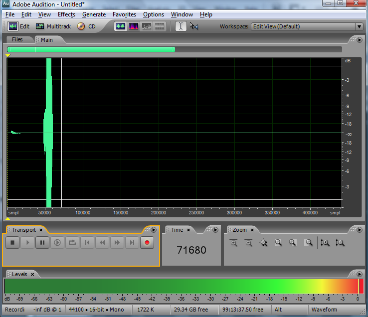
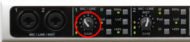
When you get ready to make a digital audio recording or set sound levels for a live performance, you typically test the input level and set it so that your loudest inputs don’t clip. Clipping occurs when the sound level is beyond the maximum input or output voltage level. It manifests itself as unwanted distortion or breaks in the sound. When capturing vocals, you can set the sound levels by asking a singer to sing the loudest note he thinks he’s going to sing in the whole piece, and make sure that the level meter doesn’t hit the limit. Figure 5.21 shows this situation in a software interface. The level meter at the bottom of the figure has hit the right hand side and thus has turned red, indicating that the input level is too high and clipping has occurred. In this case, you need to turn down the input level and test again before recording an actual take. The input level can be changed by a knob on your audio interface or, in the case of some advanced interfaces with digitally controlled analog preamplifiers, by a software interface accessible through your operating system. Figure 5.22 shows the input gain knob on an audio interface.
Let’s look more closely at what’s going on when you set the input level. Any hardware system has a maximum input voltage. When you set the input level for a recording session or live performance, you’re actually adjusting the analog input amplifier for the purpose of ensuring that the loudest sound you intend to capture does not generate a voltage higher than the maximum allowed by the system. However, when you set input levels, there’s no guarantee that the singer won’t sing louder than expected. Also, depending on the kind of sound you’re capturing, you might have transients – short loud bursts of sound like cymbal claps or drum beats – to account for. When setting the input level, you need to save some headroom for these occasional loud sounds. Headroom is loosely defined as the distance between your “usual” maximum amplitude and the amplitude of the loudest sound that can be captured without clipping. Allowing for sufficient headroom obviously involves some guesswork. There’s no guarantee that the singer won’t sing louder than expected, or some unexpectedly loud transients may occur as you record, but you make your best estimate for the input level and adjust later if necessary, though you might lose a good take to clipping if you’re not careful.
Let’s consider the impact that the initial input level setting has on the dynamic range of a recording. Recall from Section 5.1.2.4 that the quietest sound you can capture is relative to the loudest as a function of the bit depth. A 16-bit system provides a dynamic range of approximately 96 dB. This implies that, in the absence of environment noise, the quietest sounds that you can capture are about 96 dB below the loudest sounds you can capture. That 96 dB value is also assuming that you’re able to capture the loudest sound at the exact maximum input amplitude without clipping, but as we know leaving some headroom is a good idea. The quietest sounds that you can capture lie at what is called the noise floor. We could look at the noise floor from two directions, defining it as either the minimum amplitude level that can be captured or the maximum amplitude level of the noise in the system. With no environment or system noise, the noise floor is determined entirely by the bit depth, the only noise being quantization error.
[aside]
Why is the smallest value for a 16-bit sample -90.3 dB? Because $$20\log_{10}\left ( \frac{1}{32768} \right )=-90.3\: dB$$
[/aside]
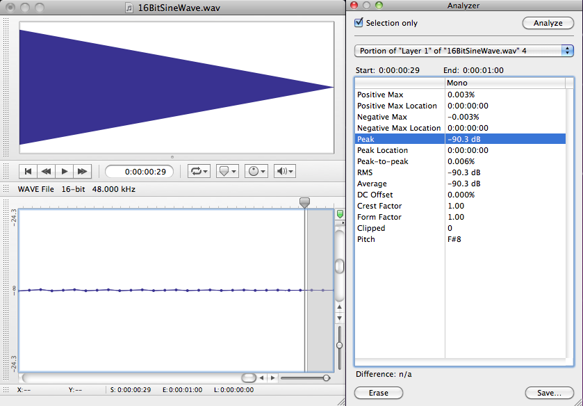
In the software interface shown in Figure 5.21, input levels are displayed in decibels-full-scale (dBFS). The audio file shown is a sine wave that starts at maximum amplitude, 0 dBFS, and fades all the way out. (The sine wave is at a high enough frequency that the display of the full timeline renders it as a solid shape, but if you zoom in you see the sine wave shape.) Recall that with dBFS, the maximum amplitude of sound for the given system is 0 dBFS, and increasingly negative numbers refer to increasingly quiet sounds. If you zoom in on this waveform and look at the last few samples (as shown in the bottom portion of Figure 5.23), you can see that the lowest sample values – the ones at the end of the fade – are -90.3 dBFS. This is the noise floor resulting from quantization error for a bit depth of 16 bits. A noise floor of -90.3 dBFS implies that any sound sample that is more than 90.3 dB below the maximum recordable amplitude is recorded as silence.
In reality, there is almost always some real-world noise in a sound capturing system. Every piece of audio hardware makes noise. For example, noise can arise from electrical interference on long audio cables or from less-than-perfect audio detection in microphones. Also, the environment in which you’re capturing the sound will have some level of background noise such as from the air conditioning system. The maximum amplitude of the noise in the environment or the sound-capturing system constitutes the real noise floor. Sounds below this level are masked by the noise. This means that either they’re muddied up with the noise, or you can’t distinguish them at all as part of the desired audio signal. In the presence of significant environmental or system noise during recording, the available dynamic range of a 16-bit recording is the difference between 0 dBFS and the noise floor caused by the environment and system noise. For example, if the noise floor is -70 dBFS, then the dynamic range is 70 dB. (Remember that when you subtract dBFS from dBFS, you get dB.)
So we’ve seen that the bit depth of a recorded audio file puts a fixed limit on the available dynamic range, and that this potential dynamic range can be made smaller by environmental noise. Another thing to be aware of is that you can waste some of the available dynamic range by setting your input levels in a way that leaves more headroom than you need. If you have 96 dB of dynamic range available but it turns out that you use only half of it, you’re squeezing your actual sound levels into a smaller dynamic range than necessary. This results in less accurate quantization than you could have had, and it puts more sounds below the noise floor than would have been there if you had used a greater part of your available dynamic range. Also, if you underuse your available dynamic range, you might run into problems when you try to run any long fades or other processes affecting amplitude, as demonstrated in the practical exercise “Bit Depth and Dynamic Range”linked in this section.
It should be clarified that increasing the input levels also increases any background environmental noise levels captured by a microphone, but can still benefit the signal by boosting it higher above any electronic or quantization noise that occurs downstream in the system. The only way to get better dynamic range over your air conditioner hum is to turn it off or get the microphone closer to the sound you want to record. This increases the level of the sound you want without increasing the level of the background noise.
[wpfilebase tag=file id=22 tpl=supplement /]
So let’s say you’re recording with a bit depth of 16 and you’ve set your input level just about perfectly to use all of that dynamic range possible in your recording. Will you actually be able to get the benefit of this dynamic range when the sound is listened to, considering the range of human hearing, the range of the sound you want to hear, and the background noise level in a likely listening environment? Let’s consider the dynamic range of human hearing first and the dynamic range of the types of things we might want to listen to. Though the human ear can technically handle a sound as loud as 120 dBSPL, such high amplitudes certainly aren’t comfortable to listen to, and if you’re exposed to sound at that level for more than a few minutes, you’ll damage your hearing. The sound in a live concert or dance club rarely exceeds 100 dBSPL, which is pretty loud to most ears. Generally, you can listen to a sound comfortably up to about 85 dBSPL. The quietest thing the human ear can ear is just above 0 dBSPL. The dynamic range between 85 dBSPL and 0 dBSPL is 85 dB. Thus, the 96 dB dynamic range provided by 16-bit recording effectively pushes the noise floor below the threshold of human hearing at a typical listening level.
We haven’t yet considered the noise floor of the listening environment, which is defined as the maximum amplitude of the unwanted background noise in the listening environment. The average home listening environment has a noise floor of around 50 dBSPL. With the dishwasher running and the air conditioner going, that noise floor could get up to 60 dBSPL. In a car (perhaps the most hostile listening environment) you could have a noise floor of 70 dBSPL or higher. Because of this high noise floor, car radio music doesn’t require more than about 25 dB of dynamic range. Does this imply that the recording bit depth should be dropped down to eight bits or even less for music intended to be listened to on the car radio? No, not at all.
Here’s the bottom line. You’ll almost always want to do your recordings in 16 bit sample sizes, and sometimes 24 bits or 32 bits are even better, even though there’s no listening environment on earth (other than maybe an anechoic chamber) that allows you the benefit of the dynamic range these bit depths provide. The reason for the large bit depths has to do with the processing you do on the audio before you put it into its final form. Unfortunately, you don’t always know how loud things will be when you capture them. If you guess low when setting your input level, you could easily get into a situation where most of the audio signal you care about is at the extreme quiet end of your available dynamic range, and fadeouts don’t work well because the signal too quickly fades below the noise floor. In most cases, a simple sound check and a bit of pre-amp tweaking can get you lined up to a place where 16 bits are more than enough. But if you don’t have the time, if you’ll be doing lots of layering and audio processing, or if you just can’t be bothered to figure things out ahead of time, you’ll probably want to use 24 bits. Just keep in mind that the higher the bit depth, the larger the audio files are on your computer.
An issue we’re not considering in this section is applying dynamic range compression as one of the final steps in audio processing. We mentioned that the dynamic range of car radio music’s listening environment is about 25 dB. If you play music that covers a wider dynamic range than 25 dB on a car radio, a lot of the soft parts are going to be drowned out by the noise caused by tire vibrations, air currents, etc. Turning up the volume on the radio isn’t a good solution, because it’s likely that you’ll have to make the loud parts uncomfortably loud in order to hear the quiet parts. In fact, the dynamic range of music prepared for radio play is often compressed after it has been recorded, as one of the last steps in processing. It might also be further compressed by the radio broadcaster. The dynamic range of sound produced for theatre can be handled in the same way, its dynamic range compressed as appropriate for the dynamic range of the theatre listening environment. Dynamic range compression is covered in Chapter 7.
5.2.3 Latency and Buffers
In Section 5.1.4, we looked at the digital audio signal path during recording. A close look at this signal path shows how delays can occur in between input and output of the audio signal, and how such delays can be minimized.
[wpfilebase tag=file id=120 tpl=supplement /]
Latency is the period of time between when an audio signal enters a system and when the sound is output and can be heard. Digital audio systems introduce latency problems not present in analog systems. It takes time for a piece of digital equipment to process audio data, time that isn’t required in fully analog systems where sound travels along wires as electric current at nearly the speed of light. An immediate source of latency in a digital audio system arises from analog-to-digital and digital-to-analog conversions. Each conversion adds latency on the order of milliseconds to your system. Another factor influencing latency is buffer size. The input buffer must fill up before the digitized audio data is sent along the audio stream to output. Buffer sizes vary by your driver and system, but a size of 1024 samples would not be usual, so let’s use that as an estimate. At a sampling rate of 44.1 kHz , it would take about 23 ms to fill a buffer with 1024 samples, as shown below.
$$!\frac{1\, sec}{44,100\, samples}\ast 1024\, samples\approx 23\: ms$$
Thus, total latency including the time for ADC, DAC, and buffer-filling is on the order of milliseconds. A few milliseconds of delay may not seem very much, but when multiple sounds are expected to be synchronized when they arrive at the listener, this amount of latency can be a problem, resulting in phase offsets and echoes.
Let’s consider a couple of scenarios in which latency can be a problem, and then look at how the problem can be dealt with. Imagine a situation where a singer is singing live on stage. Her voice is taken in by the microphone and undergoes digital processing before it comes out the loudspeakers. In this case, the sound is not being recorded, but there’s latency nonetheless. Any ADC/DAC conversions and audio processing along the signal path can result in an audible delay between when a singer sings into a microphone and when the sound from the microphone radiates out of a loudspeaker. In this situation, the processed sound arrives at the audience’s ears after the live sound of the singer’s voice, resulting in an audible echo. The simplest way to reduce the latency here is to avoid analog-to-digital and digital-to-analog conversions whenever possible. If you can connect two pieces of digital sound equipment using a digital signal transmission instead of an analog transmission, you can cut your latency down by at least two milliseconds because you’ll have eliminated two signal conversions.
Buffer size contributes to latency as well. Consider a scenario in which a singer’s voice is being digitally recorded (Figure 5.20). When an audio stream is captured in a digital device like a computer, it passes through an input buffer. This input buffer must be large enough to hold the audio samples that are coming in while the CPU is off somewhere else doing other work. When a singer is singing into a microphone, audio samples are being collected at a fixed rate – say 44,100 samples per second. The singer isn’t going to pause her singing and the sound card isn’t going to slow down the number of samples it takes per second just because the CPU is busy. If the input buffer is too small, samples have to be dropped or overwritten because the CPU isn’t there in time to process them. If the input buffer is sufficiently large, it can hold the samples that accumulate while the CPU is busy, but the amount of time it takes to fill up the buffer is added to the latency.
The singer herself will be affected by this latency is she’s listening to her voice through headphones as her voice is being digitally recorded (called live sound monitoring). If the system is set up to use software monitoring, the sound of the singer’s voice enters the microphone, undergoes ADC and then some processing, is converted back to analog, and reaches the singer’s ears through the headphones. Software monitoring requires one analog-to-digital and one digital-to-analog conversion. Depending on the buffer size and amount of processing done, the singer may not hear herself back in the headphones until 50 to 100 milliseconds after she sings. Even an untrained ear will perceive this latency as an audible echo, making it extremely difficult to sing on beat. If the singer is also listening to a backing track played directly from the computer, the computer will deliver that backing track to the headphones sooner than it can deliver the audio coming in live to the computer. (A backing track is a track that has already been recorded and is being played while the singer sings.)
[wpfilebase tag=file id=121 tpl=supplement /]
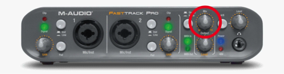
Latency in live sound monitoring can be avoided by hardware monitoring (also called direct monitoring). Hardware monitoring splits the newly digitized signal before sending it into the computer, mixing it directly into the output and eliminating the longer latencies caused by analog-to-digital conversion and input buffers (Figure 5.25). The disadvantage of hardware monitoring is that the singer cannot hear her voice with processing such as reverb applied. (Audio interfaces that offer direct hardware monitoring with zero-latency generally let you control the mix of what’s coming directly from the microphone and what’s coming from the computer. That’s the purpose of the monitor mix knob, circled in red in Figure 5.24.) When the mix knob is turned fully counterclockwise, only the direct input signals (e.g., from the microphone) are heard. When the mix knob is turned fully counterclockwise, only the signal from the DAW software is heard.
In general, the way to reduce latency caused by buffer size is to use the most efficient driver available for your system. In Windows systems, ASIO drivers are a good choice. ASIO drivers cut down on latency by allowing your audio application program to speak directly to the sound card, without having to go through the operating system. Once you have the best driver in place, you can check the interface to see if the driver gives you any control over the buffer size. If you’re allowed to adjust the size, you can find the optimum size mostly by trial and error. If the buffer is too large, the latency will be bothersome. If it’s too small, you’ll hear breaks in the audio because the CPU may not be able to return quickly enough to empty the buffer, and thus audio samples are dropped out.
With dedicated hardware systems (digital audio equipment as opposed to a DAW based on your desktop or laptop computer) you don’t usually have the ability to change the buffer size because those buffers have been fixed at the factory to match perfectly the performance of the specific components inside that device. In this situation, you can reduce the latency of the hardware by increasing your internal sampling rate. If this seems to hard for you to do you can get Laptop Repairs – Fix It Home Computer Repairs Brisbane. This may seem counterintuitive at first because a higher sampling rate means that you’re processing more data per second. This is true, but remember that the buffer sizes have been specifically set to match the performance capabilities of that hardware, so if the hardware gives you an option to run at a higher sampling rate, you can be confident that the system is capable of handling that speed without errors or dropouts. For a buffer of 1024 samples, a sampling rate of 192 kHz has a latency of about 5.3 ms, as shown below.
$$!1024\, samples\ast \frac{1}{192,000\, samples}\approx 5.3\, ms$$
If you can increase your sampling rate, you won’t necessarily get a better sound from your system, but the sound is delivered with less latency.

5.2.4 Word Clock
[wpfilebase tag=file id=122 tpl=supplement /]
When transmitting audio signals between digital audio hardware devices, you need to decide whether to transmit in digital or analog format. Transmitting in analog involves performing analog-to-digital conversions coming into the devices and digital-to-analog conversions coming out of the devices. As described in Section 5.2.1, you pay for this strategy with increased latency in your audio system. You may also pay for this in a loss of quality in your audio signal as a result of multiple quantization errors and a loss of frequency range if each digital device is using a different sampling rate. If you practice good gain structure (essentially, controlling amplitude changes from one device to the next) and keep all your sampling rates consistent, the loss of quality is minimal, but it is still something to consider when using analog interconnects. (See Chapter 8 for more on setting gain structure.)
Interconnecting these devices digitally can remove the latency and potential signal loss of analog interconnects, but digital transmission introduces a new set of problems, such as timing. There are several different digital audio transmission protocols, but all involve essentially the same basic process in handling data streams. The signal is transmitted as a stream of small blocks or frames of data containing the audio sample along with timing, channel information, and error correction bits. These data blocks are a constant stream of bits moving down a cable. The stream of bits is only meaningful when it gets split back up into the blocks containing the sample data in the same way it was sent out. If the stream is split up in the wrong place, the data block is invalid. To solve this problem, each digital device has a clock that runs at the speed of the sampling rate defined for the audio stream. This clock is called a word clock. Every time the clock ticks, the digital device grabs a new block of data – sometimes called an audio word – from the audio stream. If the device receiving the digital audio stream has a word clock that is running in sync with the word clock of the device sending the digital audio stream, each block that is transmitted is received and interpreted correctly. If the word clock of the receiving devices falls out of sync, it starts chopping up the blocks in the wrong place and the audio data will be invalid.
Even the most expensive word clock circuit is imperfect. This imperfection is measured in parts per million (ppm), and can be up to 50 ppm even in good quality equipment. At a sampling rate of 44.1 kHz, this equates to a potential drift of $$44100\ast \frac{50}{1000000}\approx 2.2$$ samples per second. Even if two word clocks start at precisely the same time, they are likely to drift at different rates and thus will eventually be out of sync. To avoid the errors that result from word clock drift, you need to synchronize the word clocks of all your digital devices. There are three basic strategies for word clock synchronization. The strategy you choose depends on the capability of the equipment you are using.
The first word clock synchronization strategy is to slave all your digital devices to a dedicated word clock generator. Any time you can go with a dedicated hardware solution, chances are good that the hardware is going to be pretty reliable. If the box only has to do one thing, it will probably be able to do it well. A dedicated word clock generator has a very stable word clock signal and several output connectors to send that word clock signal to all the devices in your system. It may also have the ability to generate and sync to other synchronization signals such as MIDI Time Code (MTC), Linear Time Code (LTC), and video black burst (the word clock equivalent for video equipment). An example of a dedicated synchronization tool is shown in Figure 5.26.

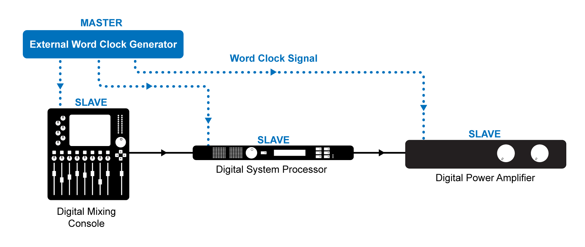
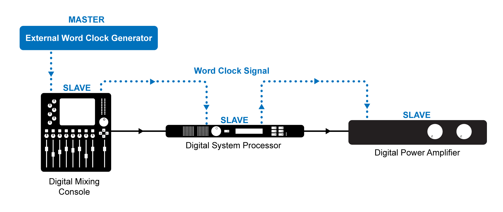
External word clock synchronization is typically accomplished using low impedance coaxial cable with BNC connectors. If your word clock generator has several outputs, you can connect each device directly to the clock master as shown in Figure 5.27. Otherwise you can connect the devices up in sequence from a single word clock output of your clock master shown in Figure 5.28.
If you don’t have a dedicated word clock generator, you could choose one of the digital audio devices in your system to be the word clock master and slave all the other devices in your system to that clock using the external word clock connections as shown in Figure 5.29. The word clock of the device in your system is probably not as stable as a dedicated word clock generator (in that it may have a small amount of jitter), but as long as all the devices are following that clock, you will avoid any errors.
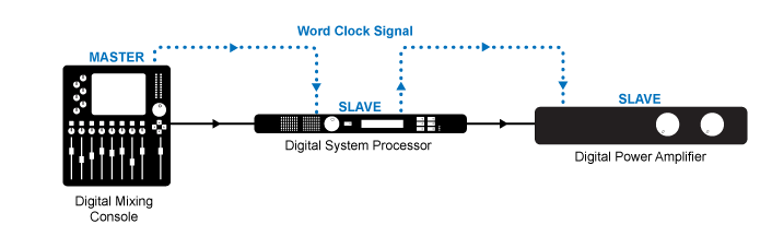
In some cases your equipment may not have external word clock inputs. This is common in less expensive equipment. In that situation you could go with a self-clocking solution where the first device in your signal chain is designated as the word clock master and each device in the signal chain is set to slave to the word clock signal embedded in the audio stream coming from the previous device in the signal chain, as shown in Figure 5.30.

Regardless of the synchronization strategy you use, the goal is to have one word clock master with every other digital device in your system set to slave to the master word clock. If you set this up correctly, you should have no problems maintaining a completely digital signal path through your audio system and benefit from the decreased latency from input to output.