4.3.1 Deriving Power and Voltage Changes in Decibels
Let’s turn now to explore more of the mathematics of concepts related to acoustics.
In Section 2, Table 4.2 lists some general guidelines regarding sound perception, and Table 4.5 gives some rules of thumb regarding power or voltage changes converted to decibels. We can’t mathematically prove the relationships in Table 4.2 because they’re based on subjective human perception, but we can prove the relationships in Table 4.5.
First let’s prove that if we double the power in watts, we get a 3 dB increase. As you work through this example, you see that you don’t always use decibels related to the reference points in Table 4.3. (That is, the standard reference point is not always the value in the denominator.) Sometimes you compare one wattage level to another, or one voltage level to another, or one sound pressure level to another, wanting to know the difference between the two in decibels. In those cases, the answer represents a difference in two wattage, voltage, or sound pressure levels, and it is measured in dB.
In general, to compare two power levels, we use the following:
[equation caption=”Equation 4.15″]
The difference in decibels between power $$P_{0}$$ and power $$P_{1}$$ = $$10\log_{10}\left ( \frac{P_{0}}{P_{1}} \right )$$
[/equation]
If $$P_{1} = 2P_{0}$$ then we have
$$!10\log_{10}\left ( \frac{2P_{0}}{P_{0}} \right )=10\log_{10}2\approx 3\: dB\: increase$$
You can illustrate this rule of thumb with two specific wattage levels – for example 1000 W and 500 W. First, convert watts to dBm. Table 4.3 gives the reference point for the definitions of dBm, dBW, dBV, an dBu. The table shows that dBM uses 0.001 W as the reference point, which means that it is in the denominator inside the log.
$$!10\log_{10}\left ( \frac{1000}{0.001} \right )=60\: dBm$$
Thus, 1000 W is 60 dBm.
What is 500 W in dBM? The standard reference point for dBm is 0.001 W. This yields.
$$!10\log_{10}\left ( \frac{500}{0.001} \right )\approx 57\: dBm$$
We see that 500 W is about 57 dBm, confirming that doubling the wattage results in a 3 dB increase, just as we predicted. We get the same result if we compute the increase in decibels based on dBW. dBW uses a reference point of 1 W in the denominator.
$$!10\log_{10}\left ( \frac{1000}{1} \right )= 30\: dBW$$
1000 W is about 30 dBW.
$$!10\log_{10}\left ( \frac{500}{1} \right )\approx 27\: dBW$$
500 W is about 27 dBW. Again, doubling the wattage results in a 3 dB increase, as predicted.
Continuing with Table 4.5, we can show that if we multiply power by 10, we have a 10 dB increase in power.
$$!10\log_{10}10= 10\: dB \:increase \:in \:power$$
If we divide the power by 10, we get a 10 dB decrease in power.
$$!10\log_{10}\left ( \frac{1}{10} \right )= -10\: dB \:decrease \:in \:power$$
For voltage, we use the formula $$20\log_{10}\left ( \frac{V_{1}}{V_{0}} \right )$$, as shown in Table 4.3. From this we can show that if we double the voltage, we have a 6 dB increase.
$$!20\log_{10}2\approx 6\: dB\: increase\: in\: voltage$$
If we multiply the voltage times 10, we get a 20 dB increase
$$!20\log_{10}10= 20\: dB\: increase\: in\: voltage$$
Don’t be fooled into thinking that if we multiply the voltage by 5, we’ll get a 10 dB increase. Instead, multiplying voltage times 5 yields about 14 dB increase in voltage.
$$!20\log_{10}5\approx 14\: dB\: increase\: in\: voltage$$
The rest of the rows in the table related to voltage can be proven similarly.
4.3.2 Working with Critical Bands
Recall from Section 1 that critical bands are areas in the human ear that are sensitive to certain bandwidths of frequencies. The presence of critical bands in our ears is responsible for the masking of frequencies that are close to other louder ones that are received by the same critical band.
In most sources, tables that estimate the widths of critical bands in human hearing give the bandwidths only in Hertz. In Table 4.4, we added two additional columns. Column 5 of Table 4.4 derives the number of semitones n in a critical band based on the beginning and ending frequencies in the band. Column 6 is the approximate size of the critical band in octaves. Let’s look at how we derived these two columns.
First, consider column 5, which gives the critical bandwidth in semitones. Chapter 3 explains that there are 12 semitones in an octave. The note at the high end of an octave has twice the frequency of a note at the low end. Thus, for frequency $$f_{2}$$ that is n semitones higher than $$f_{1}$$,
$$!f_{2}=\sqrt[12]{2}^{n}\ast f_{1}$$
To derive column 5 for each row, let b be the beginning frequency of the band, and let e be the end frequency of the band in that row. We want to find n such that
$$!e=b\ast\left ( \sqrt[12]{2} \right )^{n}$$
This equation can be simplified to find n.
$$!e=b\ast 2^{\frac{n}{12}}$$
$$!\frac{e}{b}=2^{\frac{n}{12}}$$
Table 4.7 is included to give an idea of the twelfth root of 2 and powers of it.
[table th=”0″ width=”40%”]
$$\sqrt[12]{2}^{1}=2^{\frac{1}{12}}$$,1.0595
$$\sqrt[12]{2}^{2}=2^{\frac{2}{12}}$$,1.1225
$$\sqrt[12]{3}^{3}=2^{\frac{3}{12}}$$,1.1892
$$\sqrt[12]{4}^{4}=2^{\frac{4}{12}}$$,1.2599
$$\sqrt[12]{5}^{5}=2^{\frac{5}{12}}$$,1.3348
$$\sqrt[12]{6}^{6}=2^{\frac{6}{12}}$$,1.4142
$$\sqrt[12]{7}^{7}=2^{\frac{7}{12}}$$,1.4983
$$\sqrt[12]{8}^{8}=2^{\frac{8}{12}}$$,1.5874
$$\sqrt[12]{9}^{9}=2^{\frac{9}{12}}$$,1.6818
$$\sqrt[12]{10}^{10}=2^{\frac{10}{12}}$$,1.7818
$$\sqrt[12]{11}^{11}=2^{\frac{11}{12}}$$,1.8877
$$\sqrt[12]{12}^{12}=2^{\frac{12}{12}}$$,2
[/table]
Table 4.7 Powers of $$\sqrt[12]{2}$$
Column 5 is an estimate for n rounded to the nearest integer, which is the approximate number of semitone steps from the beginning to the end of the band.
Column 6 is derived based on the n computed for column 5. If n is the number of semitones in a critical band and there are 12 semitones in an octave, then $$\frac{n}{12}$$ is the size of the critical band in octaves. Column 6 is $$\frac{n}{12}$$.
4.3.3 A MATLAB Program for Equal Loudness Contours
You may be interested in seeing how Figure 4.11 was created with a MATLAB program. The MATLAB program below is included with permission from its creator, Jeff Tacket. The program relies on data available is ISO 226. The data is given in a comment in the program. ISO is The International Organization for Standardization (www.iso.org).
figure;
[spl,freq_base] = iso226(10);
semilogx(freq_base,spl)
hold on;
for phon = 0:10:90
[spl,freq] = iso226(phon);%equal loudness data
plot(1000,phon,'.r');
text(1000,phon+3,num2str(phon));
plot(freq_base,spl);%equal loudness curve
end
axis([0 13000 0 140]);
grid on % draw grid
xlabel('Frequency (Hz)');
ylabel('Sound Pressure in Decibels');
hold off;

function [spl, freq] = iso226(phon)
% Generates an Equal Loudness Contour as described in ISO 226
% Usage:  [SPL FREQ] = ISO226(PHON);
%         PHON is the phon value in dB SPL that you want the equal
%           loudness curve to represent. (1phon = 1dB @ 1kHz)
%         SPL is the Sound Pressure Level amplitude returned for
%           each of the 29 frequencies evaluated by ISO226.
%         FREQ is the returned vector of frequencies that ISO226
%           evaluates to generate the contour.
%
% Desc:   This function will return the equal loudness contour for
%         your desired phon level.  The frequencies evaluated in this
%         function only span from 20Hz - 12.5kHz, and only 29 selective
%         frequencies are covered.  This is the limitation of the ISO
%         standard.
%
%         In addition the valid phon range should be 0 - 90 dB SPL.
%         Values outside this range do not have experimental values
%         and their contours should be treated as inaccurate.
%
%         If more samples are required you should be able to easily
%         interpolate these values using spline().
%
% Author: Jeff Tackett 03/01/05
%                /---------------------------------------\
%%%%%%%%%%%%%%%%%          TABLES FROM ISO226             %%%%%%%%%%%%%%%%%
%                \---------------------------------------/
f = [20 25 31.5 40 50 63 80 100 125 160 200 250 315 400 500 630 800 ...
1000 1250 1600 2000 2500 3150 4000 5000 6300 8000 10000 12500];

af = [0.532 0.506 0.480 0.455 0.432 0.409 0.387 0.367 0.349 0.330 0.315 ...
0.301 0.288 0.276 0.267 0.259 0.253 0.250 0.246 0.244 0.243 0.243 ...
0.243 0.242 0.242 0.245 0.254 0.271 0.301];

Lu = [-31.6 -27.2 -23.0 -19.1 -15.9 -13.0 -10.3 -8.1 -6.2 -4.5 -3.1 ...
-2.0  -1.1  -0.4   0.0   0.3   0.5   0.0 -2.7 -4.1 -1.0  1.7 ...
2.5   1.2  -2.1  -7.1 -11.2 -10.7  -3.1];

Tf = [ 78.5  68.7  59.5  51.1  44.0  37.5  31.5  26.5  22.1  17.9  14.4 ...
11.4   8.6   6.2   4.4   3.0   2.2   2.4   3.5   1.7  -1.3  -4.2 ...
-6.0  -5.4  -1.5   6.0  12.6  13.9  12.3];
%%%%%%%%%%%%%%%%%%%%%%%%%%%%%%%%%%%%%%%%%%%%%%%%%%%%%%%%%%%%%%%%%%%%%%%%%%%

%Error Trapping
if((phon < 0) || (phon > 90))
disp('Phon value out of bounds!')
spl = 0;
freq = 0;
else
%Setup user-defined values for equation
Ln = phon;

%Deriving sound pressure level from loudness level (iso226 sect 4.1)
Af=4.47E-3 * (10.^(0.025*Ln) - 1.15) + (0.4*10.^(((Tf+Lu)/10)-9 )).^af;
Lp=((10./af).*log10(Af)) - Lu + 94;

%Return user data
spl = Lp;
freq = f;
end
Program 4.1 MATLAB program for graphing equal loudness contours
4.3.4 The Mathematics of the Inverse Square Law and PAG Equations
The inverse square law says, in essence, that for two points at distance $$r_{0}$$ and $$r_{1}$$ from a point sound source, where $$r_{1}>r_{0}$$, the sound intensity diminishes by $$20\log_{10}\left ( \frac{r_{0}}{r_{1}}\right )$$ dB. To derive the inverse square law mathematically, we can use the formula for the surface area of a sphere, $$4\pi r^{2}$$, where r is the radius of the sphere. Notice that in Figure 4.18, the radius of the sphere is also the distance from the sound source to the surface of that sphere. Recall that intensity is defined as power per unit area – that is, power proportional to the area over which it is spread. As the sound gets farther from the source, it spreads out over a larger area. At any distance r from the source, $$I=\frac{P}{4\pi r^{2}}$$ where I is intensity and P is the power at the source. Notice that if you increase the radius of the sphere by a factor of n, gets smaller by a factor of $$n^{2}$$. Thus, I is proportional to the inverse of $$r^{2}$$, which can be stated mathematically as $$I \propto \frac{1}{r^{2}}$$. We can state this more completely as
[equation caption=”Equation 4.16 Ratio of sound intensity comparing one location to another”]
$$!I_{1}=I_{0}\ast \left ( \frac{r_{0}}{r_{1}} \right )^{2}$$
where $$I_{0}$$ is the intensity of the sound at the first location,
$$I_{1}$$ is the intensity of the sound at the second location,
$$r_{0}$$ is the initial distance from the sound,
and $$r_{1}$$ is the new distance from the sound.
[/equation]
We usually represent intensities in decibels, so let’s convert to decibels applying the definition of dBSIL.
$$!10\log_{10}I_{1}=10\log_{10}\left ( I_{0}\ast \left ( \frac{r_{0}}{r_{1}} \right )^{2} \right )$$
$$!10\log_{10}I_{1}=10\log_{10}I_{0}+10\log_{10}\left ( \frac{r_{0}}{r_{1}} \right )^{2}$$
Thus
[equation caption=”Equation 4.17″]
$$!I_{1\, dBSIL}-I_{0\,dBSIL}=20\log_{10}\left ( \frac{r_{0}}{r_{1}} \right )dB$$
where $$I_{0\,dBSIL}$$ is the intensity of the sound at the first location in decibels,
$$!I_{1\, dBSIL}$$ is the intensity of the sound at the second location in decibels,
$$r_{0}$$ is the initial distance from the sound,
$$r_{1}$$ and is the new distance from the sound
[/equation]
Recall that when you subtract dBSIL from dBSIL, you get dB.
Based on the inverse square law, it is easy to prove that if you double the distance from the sound, you get about a 6 dB decrease (as listed in Table 4.5).
In Section 4.2.2.1, we looked at how the PAG is determined so that a sound engineer can know the limits of the gain he can apply to the sound without getting feedback. You can understand why feedback happens and how it can be prevented by applying the inverse square law.
First, we can derive an equation for the sound level that comes from the singer arriving at the microphone at intensity $$I_{M}$$ vs. arriving at the listener at intensity $$I_{L}$$, without sound reinforcement. All sound levels are in decibels. By the inverse square law, the relationship between $$I_{L}$$and $$I_{M}$$ is this:
[equation caption=”Equation 4.18″]
$$!I_{L}-I_{M}=20\log_{10}\left ( \frac{D_{s}}{D_{0}} \right )$$
[/equation]
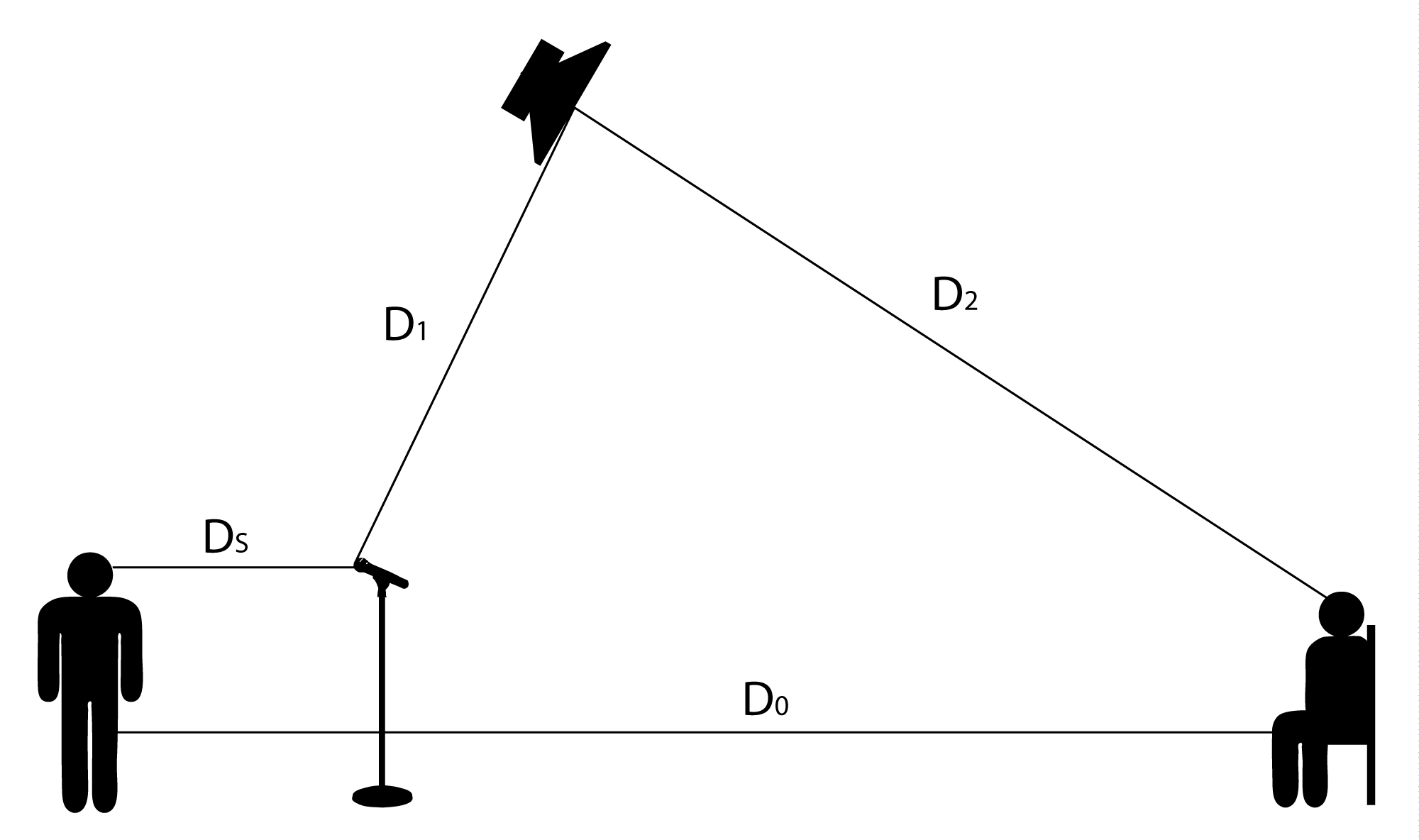
We can also apply the inverse square law to the sound coming from the loudspeaker and arriving at microphone at intensity $$I_{M’}$$ vs. arriving the listener at intensity $$I_{L’}$$, with reinforcement. Feedback occurs where $$I_{M}=I_{M’}$$. Thus we have
[equation caption=”Equation 4.19″]
$$!I_{L’}-I_{M’}=I_{L’}-I_{M}=20\log_{10}\left ( \frac{D_{1}}{D_{2}} \right )$$
[/equation]
Subtracting Equation 4.18 from Equation 4.19, we get
$$!I_{L’}-I_{L}=20\log_{10}\left ( \frac{D_{1}}{D_{2}} \right )-20\log_{10}\left ( \frac{D_{s}}{D_{0}} \right )$$
$$!I_{L’}-I_{L}=20\log_{10}\left ( \frac{\frac{D_{1}}{D_{2}}}{\frac{D_{s}}{D_{0}}} \right )$$
$$!I_{L’}-I_{L}=20\log_{10}\left ( \frac{D_{1}\ast D_{0}}{D_{s}\ast D_{2}} \right )$$
$$I_{L’}-I_{L}$$ represents the PAG, the maximum amount by which the original sound can be boosted without feedback.
$$!PAG=20\log_{10}\left ( \frac{D_{1}\ast D_{0}}{D_{s}\ast D_{2}} \right )$$
This is Equation 4.14 originally discussed in Section 4.2.2.1.
4.3.5 The Mathematics of Delays, Comb Filtering, and Room Modes
[wpfilebase tag=file id=89 tpl=supplement /]
In Section 4.2.2.4, we showed what happens when two copies of the same sound arrive at a listener at different times. For each of the frequencies in the sound, the copy of the frequency coming from speaker B is in a different phase relative to the copy coming from speaker A (Figure 4.27). In the case of frequencies that are offset by exactly one half of a cycle, the two copies of the sound are completely out-of-phase, and those frequencies are lost for the listener in that location. This is an example of comb filtering caused by delay.
To generalize this mathematically, let’s assume that loudspeaker B is d feet farther away from a listener than loudspeaker A. The speed of sound is c. Then the delay t, in seconds, is
[equation caption=”Equation 4.20 Delay t for offset d between two loudspeakers”]
$$!t=\frac{d\: ft}{c\:ft/s}$$
[/equation]
Assume for simplicity that the speed of sound is 1000 ft/s. Thus, for an offset of 20 ft, you get a delay of 0.020 s.
$$!t=\frac{20\: ft}{1000\:ft/s}$$
$$!t=0.02s=20ms$$
What if you want to know the frequencies of the sound waves that will be combed out by a delay of t? The fundamental frequency to be combed, $$f_{0}$$, is the one that is delayed by half of the period, since this delay will offset the phase of the wave by 180°. We know that the period is the inverse of the frequency, which gives us
$$!t=\frac{1}{2\ast f_{0}}$$
$$!t=\frac{1}{2\ast t}$$
Additionally, all integer multiples of $$f_{0}$$ will also be combed out, since they also will be 180° offset from the other copy of the sound. Thus, we can this formula for the frequencies combed out by delay t.
[equation caption=”Equation 4.21 Comb filtering”]
Given a delay of t seconds between two identical copies of a sound,
then the frequencies $$f_{i}$$ that will be combed out are
$$!f_{i}=\frac{i+1}{2t}for\:all\:integers\:i\geq0$$
[/equation]
[wpfilebase tag=file id=57 tpl=supplement /]
For a 20 foot separation in distance, which creates a delay of 0.02 s, the combed frequencies are 25 Hz, 50 Hz, 75 Hz, and so forth.
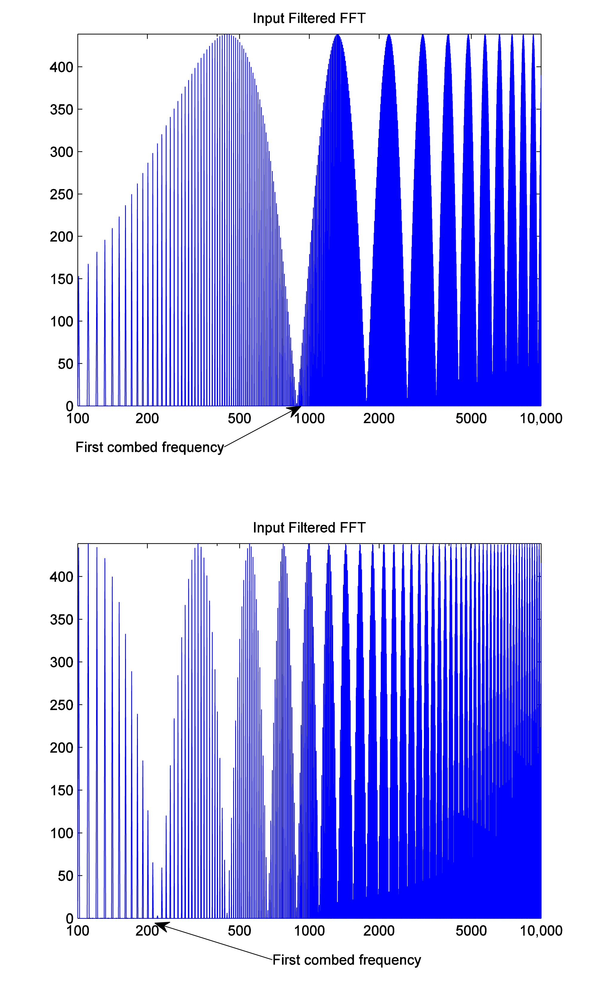
In Section 2, we made the point that comb filtering in the air can be handled by increasing the delay between the two sound sources. A 40 foot distance between two identical sound sources results in a 0.04 s delay, which then combs out 12.5 Hz, 25 Hz, 37.5 Hz, 50 Hz, and so forth. The larger delay, the lower the frequency at which combing begins, and the closer the combed frequencies are to one another. You can see this in Figure 4.41. In the first graph, a delay of 0.5682 ms combs out integer multiples of 880 Hz. In the second graph, a delay of 2.2727 ms combs out integer multiples of 220 Hz.
[wpfilebase tag=file id=17 tpl=supplement /]
If the delay is long enough, frequencies that are combed out are within the same critical band as frequencies that are amplified. Recall that all frequencies in a critical band are perceived as the same frequency. If one frequency is combed out and another is amplified within the same critical band, the resulting perceived amplitude of the frequency in that band is the same as would be heard without comb filtering. Thus, a long enough delay mitigates effect of comb filtering. The exercise associated with this section has you verify this point.
Room mode operates by the same principle as comb filtering. Picture a sound being sent from the center of a room. If the speed of sound in the room is 1000 ft/s and the room has parallel walls that are 10 feet apart, how long will it take the sound to travel from the center of the room, bounce off one of the walls, and come back to the center? Since the sound is traveling 5 + 5 =10 feet, we get a delay of $$t=\frac{10ft}{1000\frac{ft}{s}}=0.01s$$. This implies that a sound wave of frequency $$f_{0}=\frac{1}{2\ast 0.01}=50$$ Hz sound wave will be combed out in the center of the room. The center of the room is a node with regard to a frequency of 50 Hz.
[wpfilebase tag=file id=59 tpl=supplement /]
For the second harmonic, 100 Hz, the nodes are 2.5 feet from the wall. The time it takes for sound to move from a point 2.5 feet from the wall and bounce back to that same point is 2.5 + 2.5 = 5 feet, yielding a delay of $$t=\frac{5ft}{1000\frac{ft}{s}}=0.005s$$. This is half the period of the 100 Hz wave, meaning a frequency of 100 Hz will be combed out at those points. However, in the center of the room, we still have a delay of $$t=\frac{10ft}{1000\frac{ft}{s}}=0.001s$$, which is the full period of the 100 Hz wave, meaning the 100 Hz wave gets amplified at the center of the room.
The other harmonic frequencies can be explained similarly.