2.3.1 Modeling Sound in Max
Max (distributed by Cycling ‘74 and formerly called Max/MSP/Jitter) is a software environment for manipulating digital audio and MIDI data. The interface for Max is at a high level of abstraction, allowing you to patch together sound objects by dragging icons for them to a window and linking them with patcher cords, similar to the way audio hardware is connected. If you aren’t able to use Max, which is a commercial product, you can try substituting the freeware program Pure Data. We introduce you briefly to Pure Data in Section 2.3.2. In future chapters, we’ll limit our examples to Max because of its highly developed functionality, but PD is a viable free alternative that you might want to try.
[wpfilebase tag=file id=27 tpl=supplement /]
Max can be used in two ways. First, it’s an excellent environment for experimenting with sound simply to understand it better. As you synthesize and analyze sound through built-in Max objects and functions, you develop a better understanding of the event-driven nature of MIDI versus the streaming data nature of digital audio, and you see more closely how these kinds of data are manipulated through transforms, effects processors, and the like. Secondly, Max is actually used in the sound industry. When higher level audio processing programs like Logic, Pro Tools, Reason, or Sonar don’t meet the specific needs of audio engineers, they can create specially-designed systems using Max.
Max is actually a combination of two components that can be made to work together. Max allows you to work with MIDI objects, and MSP is designed for digital audio objects. Since we won’t go into depth in MIDI until Chapter 6, we’ll just look at MSP for now.
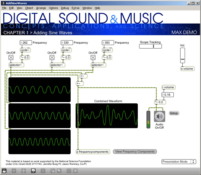
Let’s try a simple example of MSP to get you started. Figure 2.38 shows an MSP patcher for adding three pure sine waves. A patcher – whether it has Max objects, MSP objects, or both – is a visual representation of a program that operates on sound. The objects are connected by patch cords. These cords run between the inlets and outlets of objects.
One of the first things you’ll probably want to do in MSP is create simple sine waves and listen to them. To be able to work on a patcher, you have to be in edit mode, as opposed to lock mode. You enter edit mode by clicking CTRL-E (or Apple-E) or by clicking the lock icon on the task bar. Once in edit mode, you can click on the + icon on the task bar, which gives you a menu of objects. (We refer you to the Max Help for details on inserting various objects.) The cycle~ object creates a sine wave of whatever frequency you specify.
Notice that MSP objects are distinguished from Max objects by the tilde at the end of their names. This reminds you that MSP objects send audio data streaming continuously through them, while Max objects typically are triggered by and trigger discrete events.
The speaker icon in Figure 2.24 represents the ezdac~ object, which stands for “easy digital to analog conversion,” and sends sound to the sound card to be played. A number object sends the desired frequency to each cycle~ object, which in turn sends the sine wave to a scope~ object (the sine wave graphs) for display. The three frequencies are summed with two consecutive +~ objects, and the resulting complex waveform is displayed.
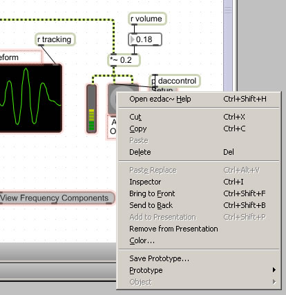
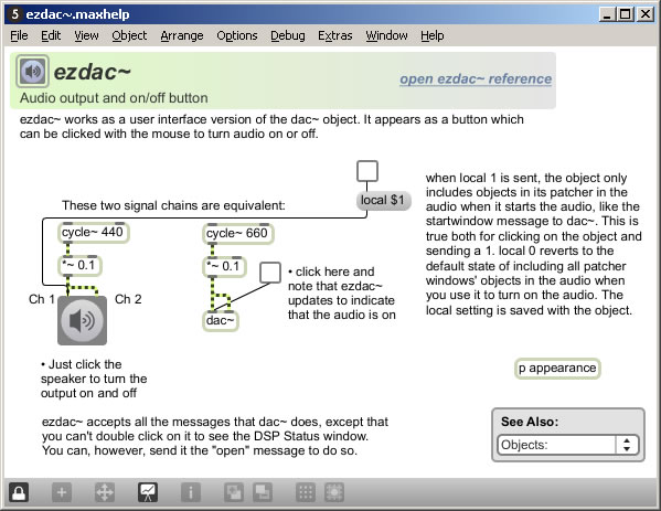
To understand these objects and functions in more detail, you can right click on them to get an Inspector window, which shows the parameters of the objects. Figure 2.25 shows the inspector for the meter~ object, which looks like an LED and is to the left of the Audio On/Off switch in Figure 2.24. You can change the parameters in the Inspector as you wish. You also can right click on an object, go to the Help menu (Figure 2.26), and access an example patcher that helps you with the selected object. Figure 2.27 shows the Help patcher for the ezdac~ object. The patchers in the Help can be run as programs, opened in Edit mode, and copied and pasted into your own patchers.

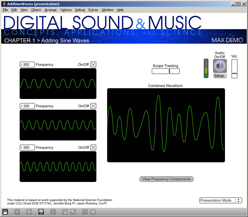
When you create a patcher, you may want to define how it looks to the user in what is called presentation mode, a view in which you can hide some of the implementation details of the patcher to make its essential functionality clearer. The example patcher’s presentation mode is shown in Figure 2.28.
2.3.2 Modeling Sound Waves in Pure Data (PD)
Pure Data (aka PD) is a free alternative to Max developed by one of the originators of Max, Miller Puckette, and his collaborators. Like Max, it is a graphical programming environment that links digital audio and MIDI.
The Max program to add sine waves is implemented in PD in Figure 2.29. You can see that the interface is very similar to Max’s, although PD has fewer GUI components and no presentation mode.
2.3.3 Modeling Sound in MATLAB
It’s easy to model and manipulate sound waves in MATLAB, a mathematical modeling program. If you learn just a few of MATLAB’s built-in functions, you can create sine waves that represent sounds of different frequencies, add them, plot the graphs, and listen to the resulting sounds. Working with sound in MATLAB helps you to understand the mathematics involved in digital audio processing. In this section, we’ll introduce you to the basic functions that you can use for your work in digital sound. This will get you started with MATLAB, and you can explore further on your own. If you aren’t able to use MATLAB, which is a commercial product, you can try substituting the freeware program Octave. We introduce you briefly to Octave in Section 2.3.5. In future chapters, we’ll limit our examples to MATLAB because it is widely used and has an extensive Signal Processing Toolbox that is extremely useful in sound processing. We suggest Octave as a free alternative that can accomplish some, but not all, of the examples in remaining chapters.
Before we begin working with MATLAB, let’s review the basic sine functions used to represent sound. In the equation y = Asin(2πfx + θ), frequency f is assumed to be measured in Hertz. An equivalent form of the sine function, and one that is often used, is expressed in terms of angular frequency, ω, measured in units of radians/s rather than Hertz. Since there are 2π radians in a cycle, and Hz is cycles/s, the relationship between frequency in Hertz and angular frequency in radians/s is as follows:
[equation caption=”Equation2.7″]Let f be the frequency of a sine wave in Hertz. Then the angular frequency, ω, in radians/s, is given by
$$!\omega =2\pi f$$
[/equation]
We can now give an alternative form for the sine function.
[equation caption=”Equation 2.8″]A single-frequency sound wave with angular frequency ω, amplitude , and A phase θ is represented by the sine function
$$!y=A\sin \left ( \omega t+\theta \right )$$
[/equation]
In our examples below, we show the frequency in Hertz, but you should be aware of these two equivalent forms of the sine function. MATLAB’s sine function expects angular frequency in Hertz, so f must be multiplied by 2π.
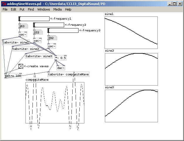
Now let’s look at how we can model sounds with sine functions in MATLAB. Middle C on a piano keyboard has a frequency of approximately 262 Hz. To create a sine wave in MATLAB at this frequency and plot the graph, we can use the fplot function as follows:
fplot('sin(262*2*pi*t)', [0, 0.05, -1.5, 1.5]);
The graph in Figure 2.30 pops open when you type in the above command and hit Enter. Notice that the function you want to graph is enclosed in single quotes. Also, notice that the constant π is represented as pi in MATLAB. The portion in square brackets indicates the limits of the horizontal and vertical axes. The horizontal axis goes from 0 to 0.05, and the vertical axis goes from –1.5 to 1.5.
If we want to change the amplitude of our sine wave, we can insert a value for A. If A > 1, we may have to alter the range of the vertical axis to accommodate the higher amplitude, as in
fplot('2*sin(262*2*pi*t)', [0, 0.05, -2.5, 2.5]);
After multiplying by A=2 in the statement above, the top of the sine wave goes to 2 rather than 1.
To change the phase of the sine wave, we add a value θ. Phase is essentially a relationship between two sine waves with the same frequency. When we add θ to the sine wave, we are creating a sine wave with a phase offset of θ compared to a sine wave with phase offset of 0. We can show this by graphing both sine waves on the same graph. To do so, we graph the first function with the command
fplot('2*sin(262*2*pi*t)', [0, 0.05, -2.5, 2.5]);
We then type
hold on
This will cause all future graphs to be drawn on the currently open figure. Thus, if we type
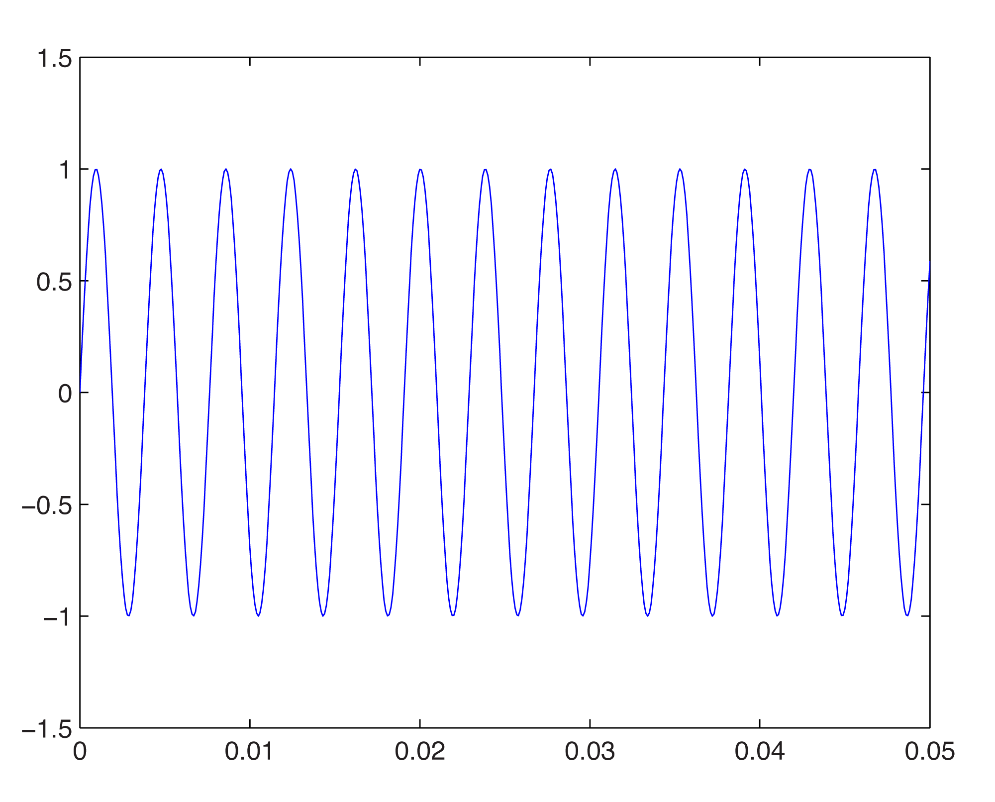
fplot('2*sin(262*2*pi*t+pi)', [0, 0.05, -2.5, 2.5]);
we have two phase-offset graphs on the same plot. In Figure 2.31, the 0-phase-offset sine wave is in red and the 180o phase offset sine wave is in blue.
Notice that the offset is given in units of radians rather than degrees, 180o being equal to radians.
To change the frequency, we change ω. For example, changing ω to 440*2*pi gives us a graph of the note A above middle C on a keyboard.
fplot('sin(440*2*pi*t)', [0, 0.05, -1.5, 1.5]);
The above command gives this graph:
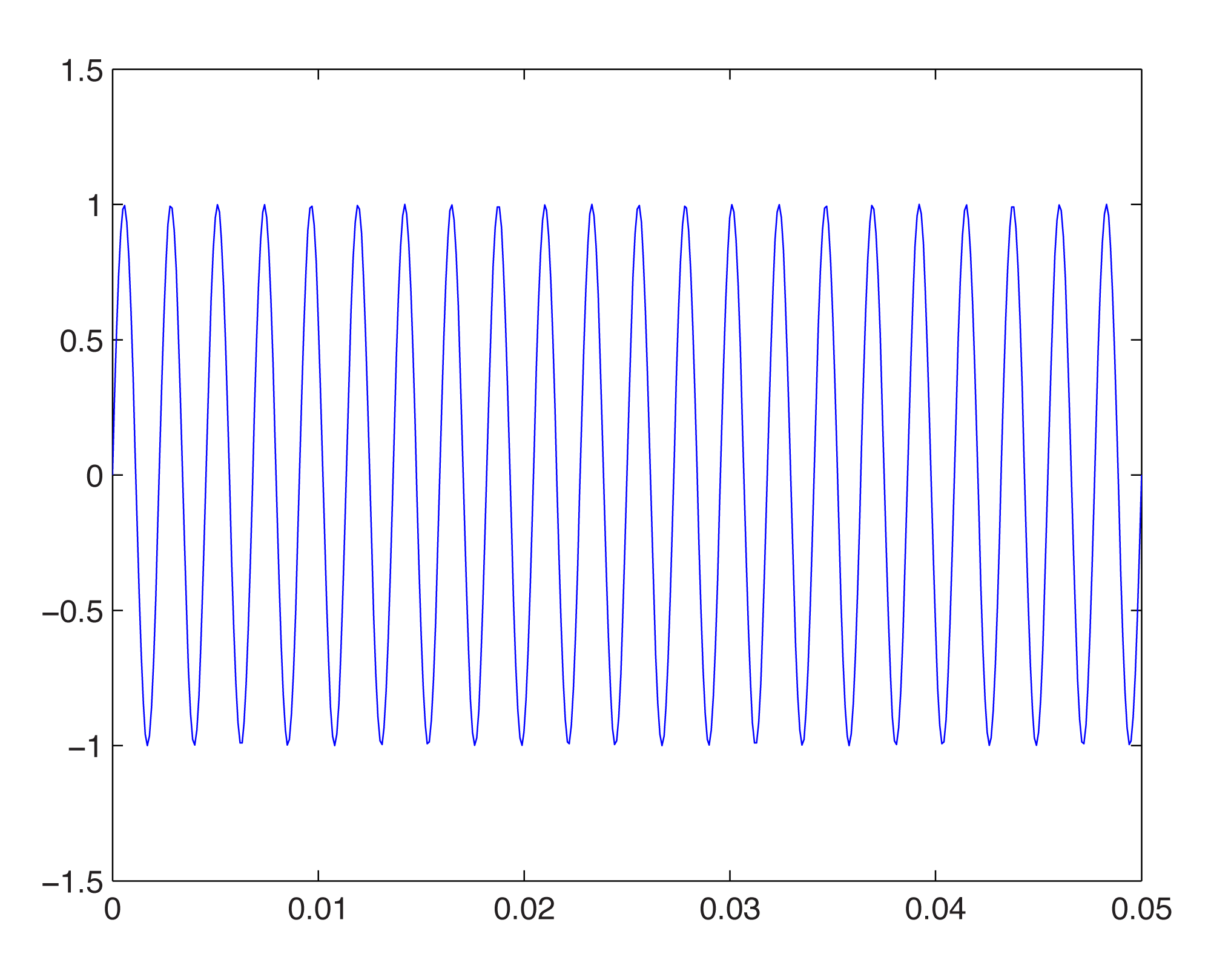
Then with
fplot('sin(262*2*pi*t)', [0, 0.05, -1.5, 1.5], 'red');

hold on
we get this figure:
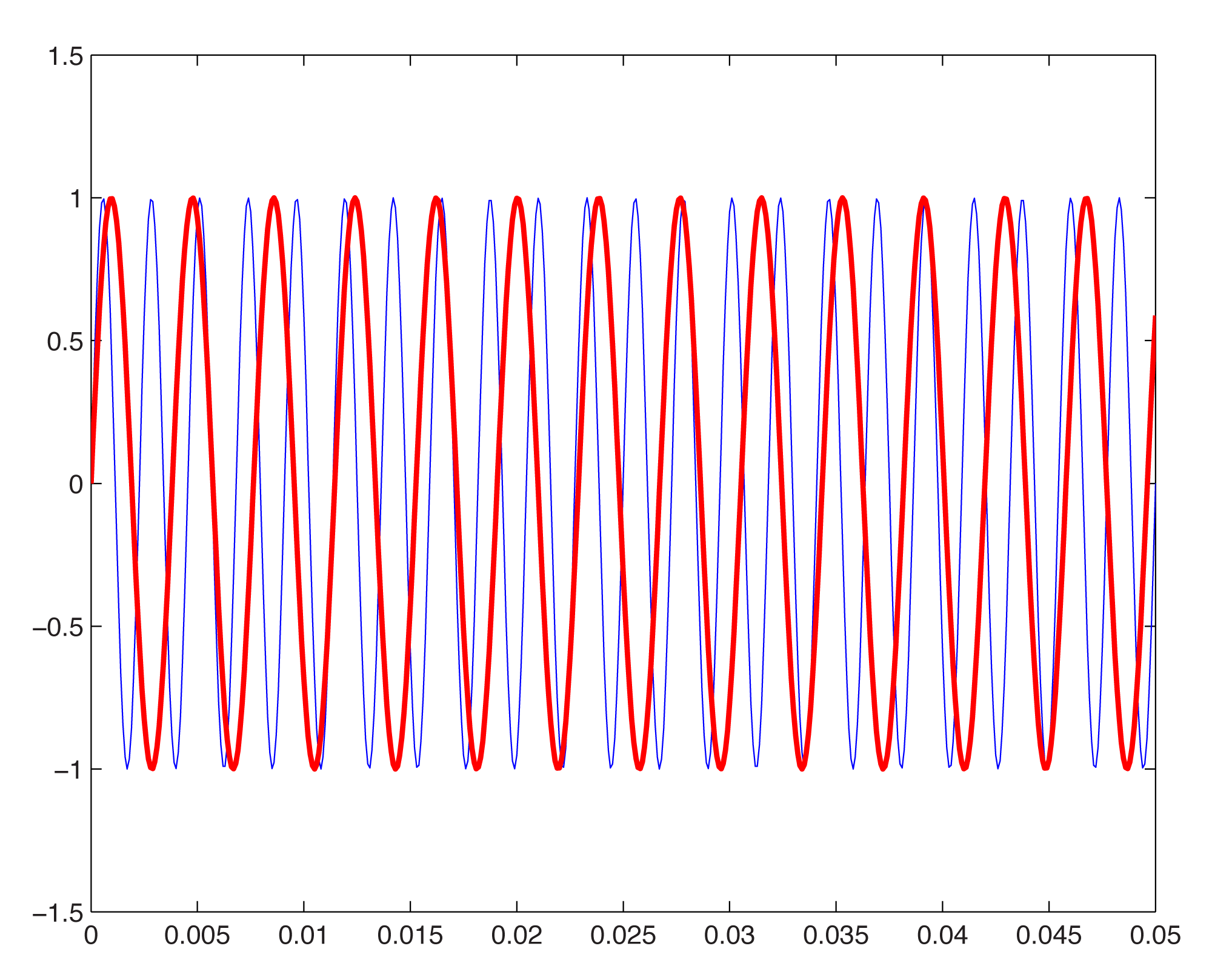
The 262 Hz sine wave in the graph is red to differentiate it from the blue 440 Hz wave.
The last parameter in the fplot function causes the graph to be plotted in red. Changing the color or line width also can be done by choosing Edit/Figure Properties on the figure, selecting the sine wave, and changing its properties.
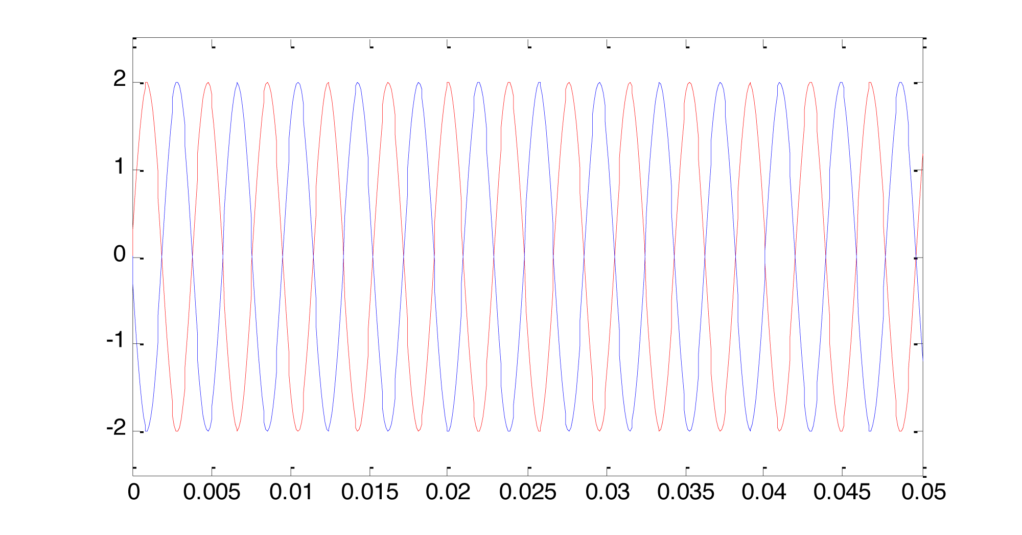
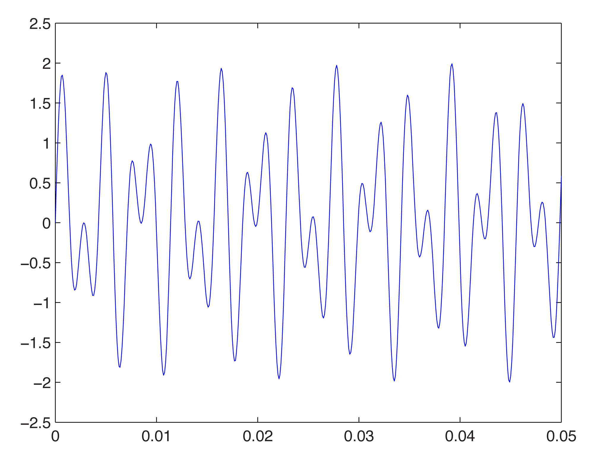
We also can add sine waves to create more complex waves, as we did using Adobe Audition in Section 2.2.2. This is a simple matter of adding the functions and graphing the sum, as shown below.
figure

fplot('sin(262*2*pi*t)+sin(440*2*pi*t)', [0, 0.05, -2.5, 2.5]);
First, we type figure to open a new empty figure (so that our new graph is not overlaid on the currently open figure). We then graph the sum of the sine waves for the notes C and A. The result is this:
We’ve used the fplot function in these examples. This function makes it appear as if the graph of the sine function is continuous. Of course, MATLAB can’t really graph a continuous list of numbers, which would be infinite in length. The name MATLAB, in fact, is an abbreviation of “matrix laboratory.” MATLAB works with arrays and matrices. In Chapter 5, we’ll explain how sound is digitized such that a sound file is just an array of numbers. The plot function is the best one to use in MATLAB to graph these values. Here’s how this works.
First, you have to declare an array of values to use as input to a sine function. Let’s say that you want one second of digital audio at a sampling rate of 44,100 Hz (i.e., samples/s) (a standard sampling rate). Let’s set the values of variables for sampling rate sr and number of seconds s, just to remind you for future reference of the relationship between the two.
sr = 44100;
s = 1;
Now, to give yourself an array of time values across which you can evaluate the sine function, you do the following:
t = linspace(0,s, sr*s);
This creates an array of sr * s values evenly-spaced between and including the endpoints. Note that when you don’t put a semi-colon after a command, the result of the command is displayed on the screen. Thus, without a semi-colon above, you’d see the 44,100 values scroll in front of you.
To evaluate the sine function across these values, you type
y = sin(2*pi*262*t);
One statement in MATLAB can cause an operation to be done on every element of an array. In this example, y = sin(2*pi*262*t) takes the sine on each element of array t and stores the result in array y. To plot the sine wave, you type
plot(t,y);
Time is on the horizontal axis, between 0 and 1 second. Amplitude of the sound wave is on the vertical axis, scaled to values between -1 and 1. The graph is too dense for you to see the wave properly. There are three ways you can zoom in. One is by choosing Axes Properties from the graph’s Edit menu and then resetting the range of the horizontal axis. The second way is to type an axis command like the following:
axis([0 0.1 -2 2]);
This displays only the first 1/10 of a second on the horizontal axis, with a range of -2 to 2 on the vertical axis so you can see the shape of the wave better.
You can also ask for a plot of a subset of the points, as follows:
plot(t(1:1000),y(1:1000));
The above command plots only the first 1000 points from the sine function. Notice that the length of the two arrays must be the same for the plot function, and that numbers representing array indices must be positive integers. In general, if you have an array t of values and want to look at only the ith to the jth values, use t(i:j).
An advantage of generating an array of sample values from the sine function is that with that array, you actually can hear the sound. When you send the array to the wavplay or sound function, you can verify that you’ve generated one second’s worth of the frequency you wanted, middle C. You do this with
wavplay(y, sr);
(which works on Windows only) or, more generally,
sound(y, sr);
The first parameter is an array of sound samples. The second parameter is the sampling rate, which lets the system know how many samples to play per second.
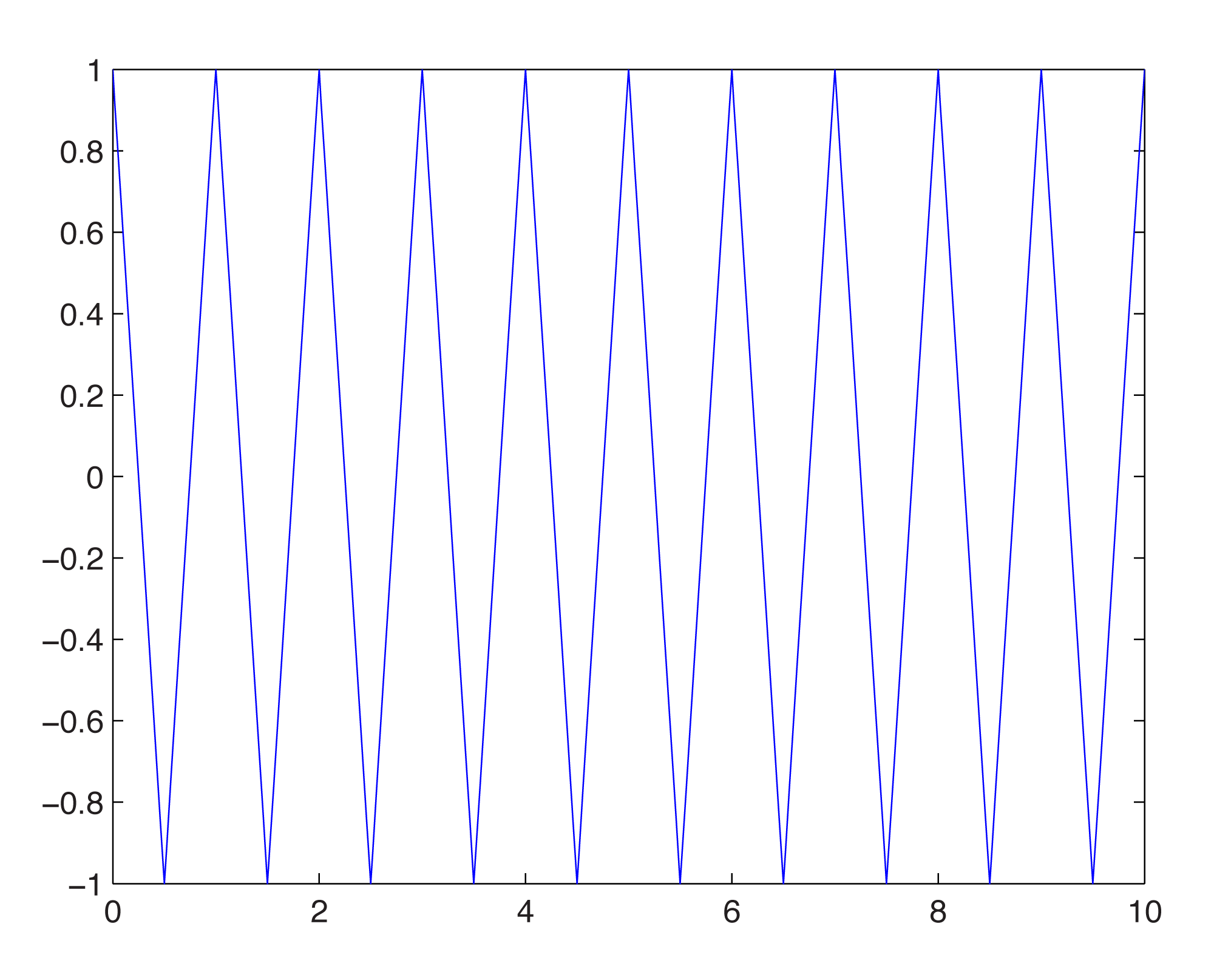
MATLAB has other built-in functions for generating waves of special shapes. We’ll go back to using fplot for these. For example, we can generate square, sawtooth, and triangular waves with the three commands given below:
fplot('square(t)',[0,10*pi,-1.5,1.5]);
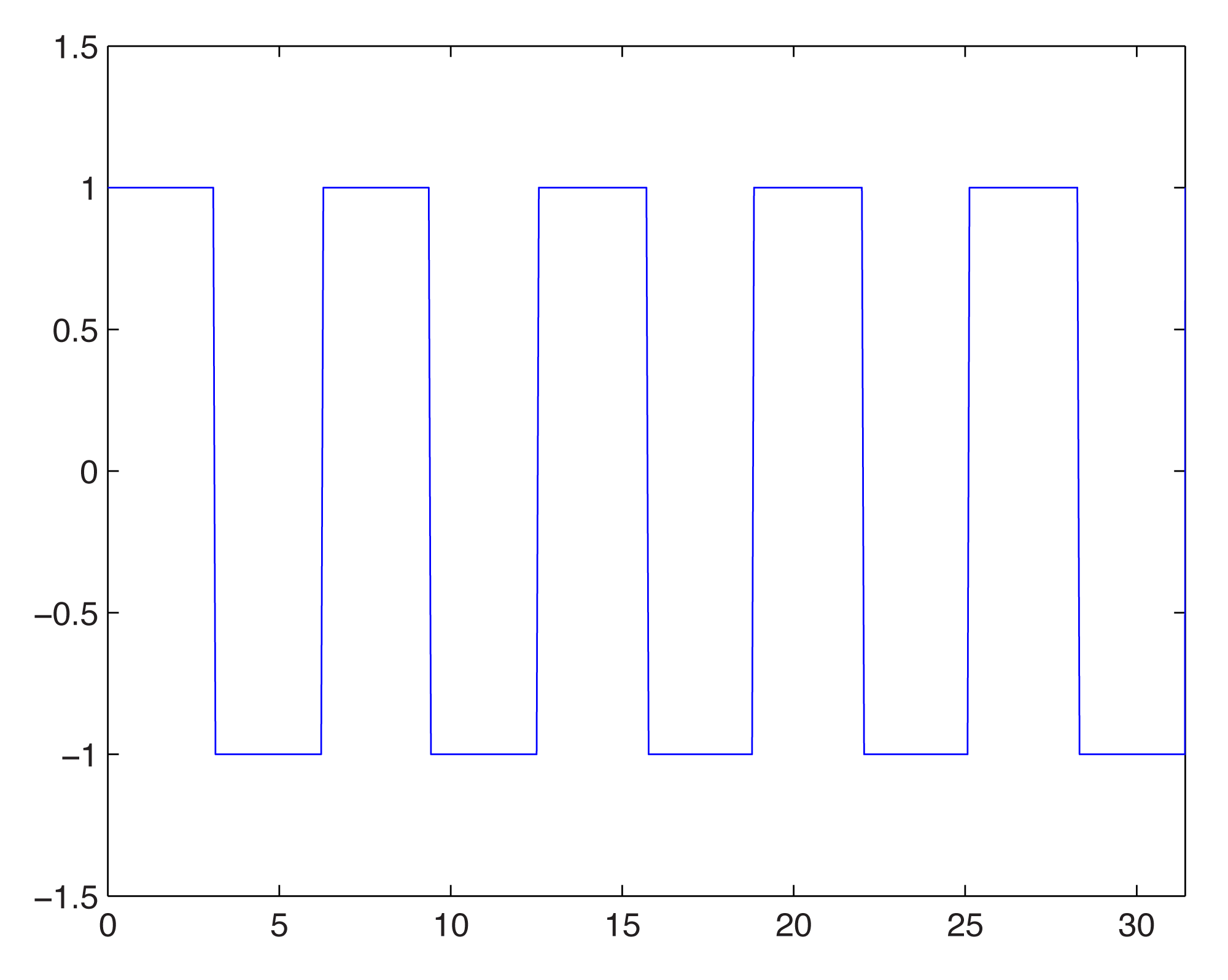
fplot('sawtooth(t)',[0,10*pi]);
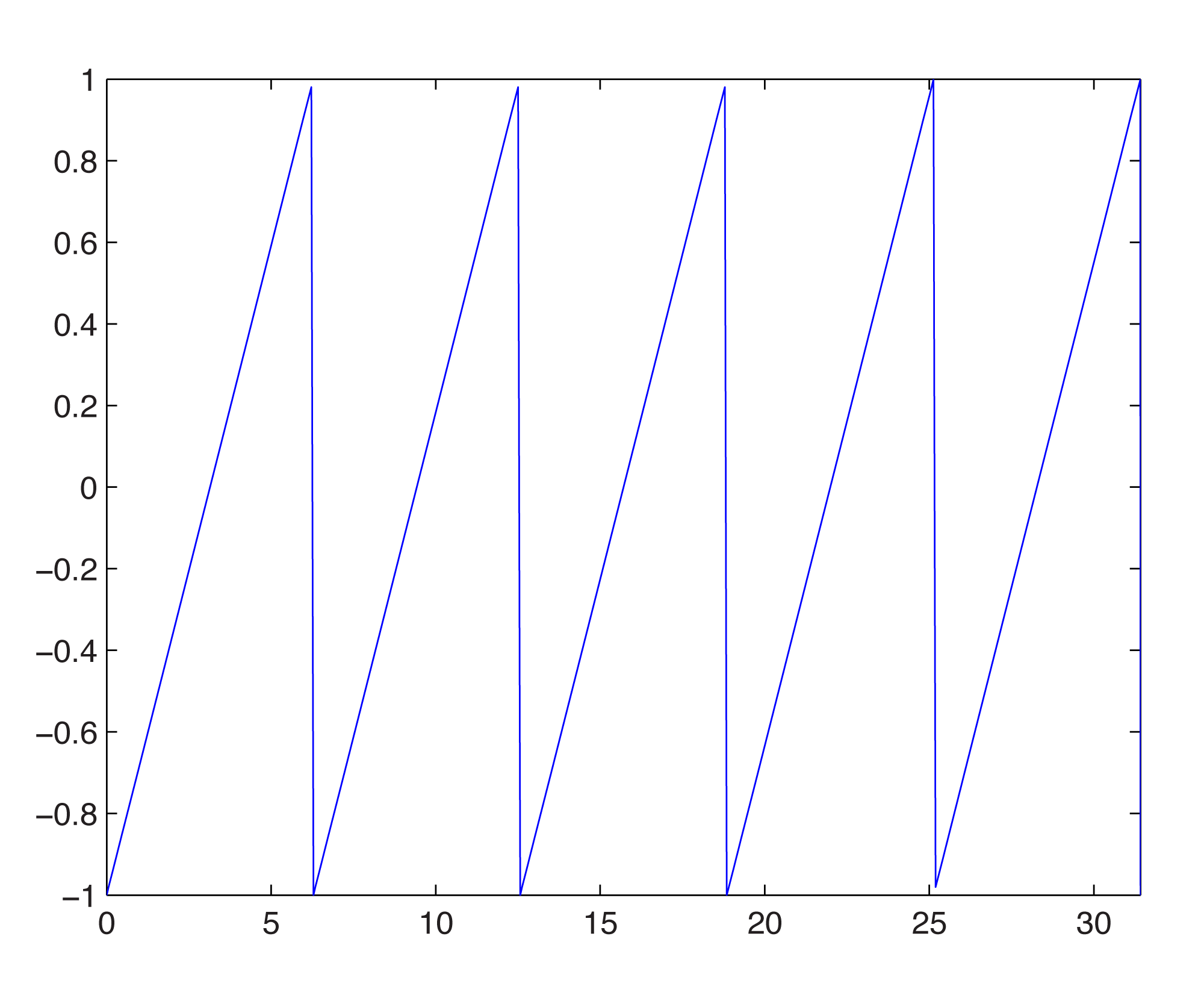
fplot('2*pulstran(t,[0:10],''tripuls'')-1',[0,10]);
(Notice that the tripuls parameter is surrounded by two single quotes on each side.)
This section is intended only to introduce you to the basics of MATLAB for sound manipulation, and we leave it to you to investigate the above commands further. MATLAB has an extensive Help feature which gives you information on the built-in functions.
Each of the functions above can be created “from scratch” if you understand the nature of the non-sinusoidal waves. The ideal square wave is constructed from an infinite sum of odd-numbered harmonics of diminishing amplitude. More precisely, if f is the fundamental frequency of the non-sinusoidal wave to be created, then a square wave is constructed by the following infinite summation:
[equation caption=”Equation 2.9″]Let f be a fundamental frequency. Then a square wave created from this fundamental frequency is defined by the infinite summation
$$!\sum_{n=0}^{\infty }\frac{1}{\left ( 2n+1 \right )}\sin \left ( 2\pi \left ( 2n+1 \right )ft \right )$$
[/equation]
Of course, we can’t do an infinite summation in MATLAB, but we can observe how the graph of the function becomes increasingly square as we add more terms in the summation. To create the first four terms and plot the resulting sum, we can do
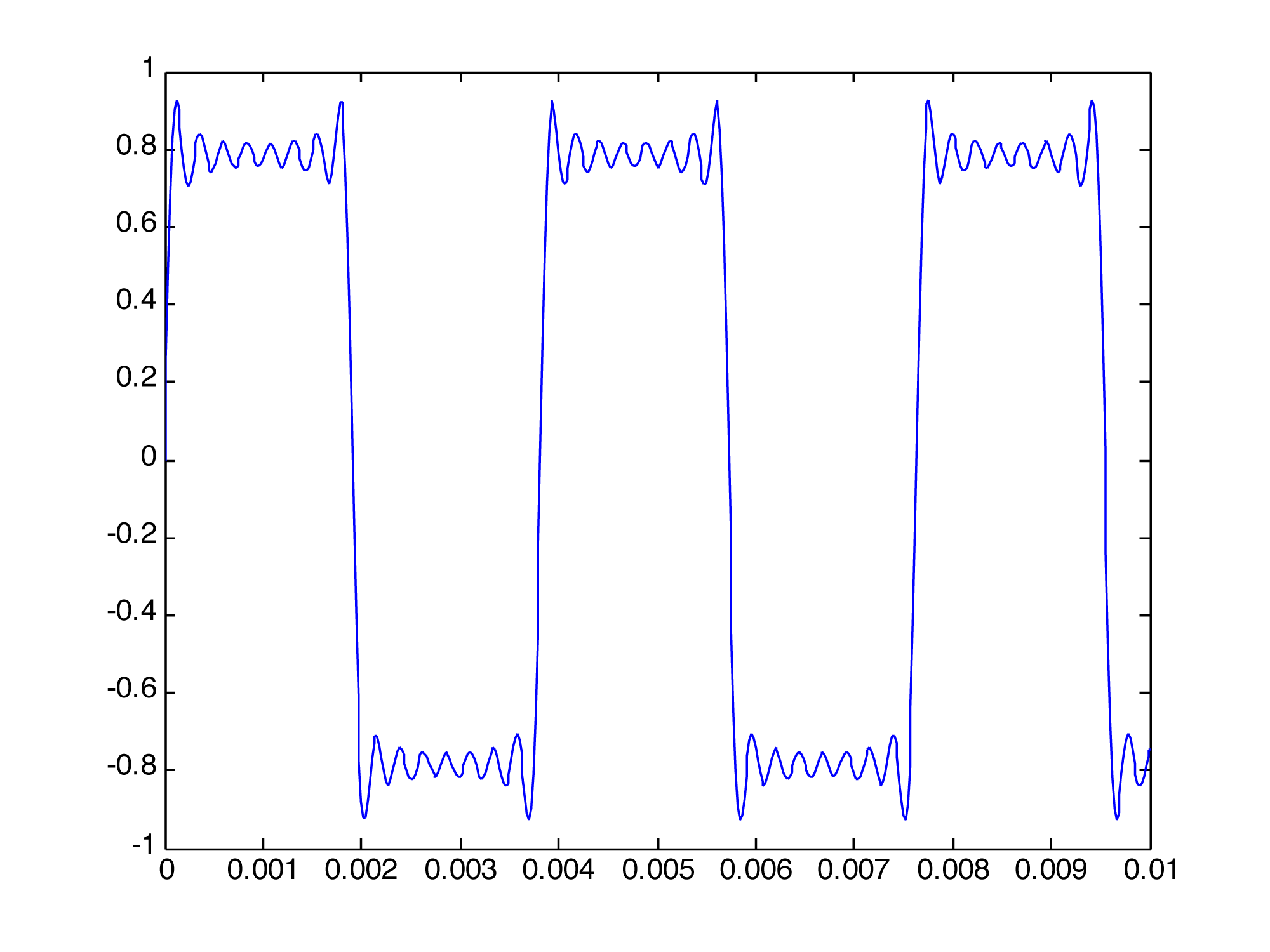
f1 = 'sin(2*pi*262*t) + sin(2*pi*262*3*t)/3 + sin(2*pi*262*5*t)/5 + sin(2*pi*262*7*t)/7';

fplot(f1, [0 0.01 -1 1]);
This gives the wave in Figure 2.38.

You can see that it is beginning to get square but has many ripples on the top. Adding four more terms gives further refinement to the square wave, as illustrated in Figure 2.39:
Creating the wave in this brute force manner is tedious. We can make it easier by using MATLAB’s sum function and its ability to do operations on entire arrays. For example, you can plot a 262 Hz square wave using 51 terms with the following MATLAB command:
fplot('sum(sin(2*pi*262*([1:2:101])*t)./([1:2:101]))',[0 0.005 -1 1])
The array notation [1:2:101] creates an array of 51 points spaced two units apart – in effect, including the odd harmonic frequencies in the summation and dividing by the odd number. The sum function adds up these frequency components. The function is graphed over the points 0 to 0.005 on the horizontal axis and –1 to 1 on the vertical axis. The ./ operation causes the division to be executed element by element across the two arrays.
The sawtooth wave is an infinite sum of all harmonic frequencies with diminishing amplitudes, as in the following equation:
[equation caption”Equation 2.10″]Let f be a fundamental frequency. Then a sawtooth wave created from this fundamental frequency is defined by the infinite summation
$$!\frac{2}{\pi }\sum_{n=1}^{\infty }\frac{\sin \left ( 2\pi n\, ft \right )}{n}$$
[/equation]
2/π is a scaling factor to ensure that the result of the summation is in the range of -1 to 1.
The sawtooth wave can be plotted by the following MATLAB command:
fplot('-sum((sin(2*pi*262*([1:100])*t)./([1:100])))',[0 0.005 -2 2])
The triangle wave is an infinite sum of odd-numbered harmonics that alternate in their signs, as follows:
[equation caption=”Equation 2.11″]Let f be a fundamental frequency. Then a triangle wave created from this fundamental frequency is defined by the infinite summation
$$!\frac{8}{\pi ^{2}}\sum_{n=0}^{\infty }\left ( \frac{sin\left ( 2\pi \left ( 4n+1 \right )ft \right )}{\left ( 4n+1 \right )^{2}} \right )-\left ( \frac{\sin \left ( 2\pi \left ( 4n+3 \right )ft \right )}{\left ( 4n+3 \right )^{2}} \right )$$
[/equation]
8/π^2 is a scaling factor to ensure that the result of the summation is in the range of -1 to 1.
We leave the creation of the triangle wave as a MATLAB exercise.
[wpfilebase tag=file id=51 tpl=supplement /]
If you actually want to hear one of these waves, you can generate the array of audio samples with
s = 1;

sr = 44100;

t = linspace(0, s, sr*s);

y = sawtooth(262*2*pi*t);
and then play the wave with
sound(y, sr);
It’s informative to create and listen to square, sawtooth, and triangle waves of various amplitudes and frequencies. This gives you some insight into how these waves can be used in sound synthesizers to mimic the sounds of various instruments. We’ll cover this in more detail in Chapter 6.
In this chapter, all our MATLAB examples are done by means of expressions that are evaluated directly from MATLAB’s command line. Another way to approach the problems is to write programs in MATLAB’s scripting language. We leave it to the reader to explore MATLAB script programming, and we’ll have examples in later chapters.
2.3.4 Reading and Writing WAV Files in MATLAB
In the previous sections, we generated sine waves to generate sound data and manipulate it in various ways. This is useful for understanding basic concepts regarding sound. However, in practice you have real-world sounds that have been captured and stored in digital form. Let’s look now at how we can read audio files in MATLAB and perform operations on them.
We’ve borrowed a short WAV file from Adobe Audition’s demo files, reducing it to mono rather than stereo. MATLAB’s audioread function imports WAV files, as follows:
y = audioread('HornsE04Mono.wav');
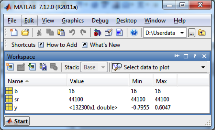
This reads an array of audio samples into y, assuming that the file is in the current folder of MATLAB. (You can set this through the Current Folder window at the top of MATLAB.) If you want to know the sampling rate and bit depth (the number of bits per sample) of the audio file, you can get this information with
[y, sr, b] = audioread('HornsE04Mono.wav');
sr now contains the sampling rate and b contains the bit depth. The Workspace window shows you the values in these variables.
You can play the sound with
sound(y, sr);
Once you’ve read in a WAV file and have it stored in an array, you can easily do mathematical operations on it. For example, you can make it quieter by multiplying by a number less than 1, as in
y = y * 0.5;
You can also write out the new form of the sound file, as in
audiowrite('HornsNew.wav', y, 44100);
2.3.5 Modeling Sound in Octave
Octave is a freeware, open-source version of MATLAB distributed by GNU. It has many but not all of the functions of MATLAB. There are versions of Octave for Linux, UNIX, Windows, and Mac OS X.
If you try to do the above exercise in Octave, most of the functions are the same. The fplot function is the same in Octave as in MATLAB except that for colors, you must put a digit from 0 to 7 in single quotes rather than use the name of the color. The linspace function is the same in Octave as in MATLAB. To play the sound, you need to use the playsound function rather than wavplay. You also can use a wavwrite function (which exists in both MATLAB and Octave) to write the audio data to an external file. Then you can play the sound with your favorite media player.
There is no square or sawtooth function in Octave. To create your own sawtooth, square, or triangle wave in Octave, you can use the Octave programs below. You might want to consider why the mathematical shortcuts in these programs produced the desired waveforms.
function saw = sawtooth(freq, samplerate)

x = [0:samplerate];
wavelength = samplerate/freq;
saw = 2*mod(x, wavelength)/wavelength-1;

end
Program 2.1 Sawtooth wave in Octave
function sqwave = squarewave(freq, samplerate)

x = [0:samplerate];
wavelength = samplerate/freq;
saw = 2*mod(x, wavelength)/wavelength-1; %start with sawtooth wave
sawzeros = (saw == zeros(size(saw))); %elminates division by zero in next step
sqwave = -abs(saw)./(saw+sawzeros); %./ for element-by-element division

end
Program 2.2 Square wave in Octave
function triwave = trianglewave(freq, samplerate)

x = [0:samplerate];
wavelength = samplerate/freq;
saw = 2*mod(x, wavelength)/wavelength-1; %start with sawtooth wave
tri = 2*abs(saw)-1;

end
Program 2.3 Triangle wave in Octave
2.3.6 Transforming from One Domain to Another
In Section 2.2.3, we showed how sound can be represented graphically in two ways. In the waveform view, time is on the horizontal axis and amplitude of the sound wave is on the vertical axis. In the frequency analysis view, frequency is on the horizontal axis and the magnitude of the frequency component is on the vertical axis. The waveform view represents sound in the time domain. The frequency analysis view represents sound in the frequency domain. (See Figure 2.18 and Figure 2.19.) Whether sound is represented in the time or the frequency domain, it’s just a list of numbers. The information is essentially the same – it’s just that the way we look at it is different.
The one-dimensional Fourier transform is function that maps real to the complex numbers, given by the equation below. It can be used to transform audio data from the time to the frequency domain.
[equation caption=”Equation 2.12 Fourier transform (continuous)”]
$$!F\left ( n \right )=\int_{-\infty }^{\infty }f\left ( k \right )e^{-i2\pi nk}dk\: where\: i=\sqrt{-1}$$
[/equation]
Sometimes it’s more convenient to represent sound data one way as opposed to another because it’s easier to manipulate it in a certain domain. For example, in the time domain we can easily change the amplitude of the sound by multiplying each amplitude by a number. On the other hand, it may be easier to eliminate certain frequencies or change the relative magnitudes of frequencies if we have the data represented in the frequency domain.
2.3.7 The Discrete Fourier Transfer and its Inverse
To be applied to discrete audio data, the Fourier transform must be rendered in a discrete form. This is given in the equation for the discrete Fourier transform below.
[equation caption=”Equation 2.13 Discrete Fourier transform”]
$$!F_{n}=\frac{1}{N}\left ( \sum_{k-0}^{N-1}f_{k}\cos \frac{2\pi nk}{N}-if_{k}\sin \frac{2\pi nk}{N} \right )=\frac{1}{N}\left ( \sum_{k=0}^{N-1}f_{k}e^{\frac{-i2\pi kn}{N}} \right )\mathrm{where}\; i=\sqrt{-1}$$
[/equation]
[aside]
The second form of the discrete Fourier transform given in Equation 2.1, $$\frac{1}{N}\left (\sum_{k=0}^{N-1}f_{k}e^{\frac{-i2\pi kn}{N}} \right )$$, uses the constant e. It is derivable from the first by application of Euler’s identify, $$e^{i2\pi kn}=\cos \left ( 2\pi kn \right )+i\sin \left ( 2\pi kn \right )$$. To see the derivation, see (Burg 2008).
[/aside]
Notice that we’ve switched from the function notation used in Equation 2.12 ( $$F\left ( n \right )$$ and F\left ( k \right )) to array index notation in Equation 2.13 ( F_{n} and f_{k}) to emphasize that we are dealing with an array of discrete audio sample points in the time domain. Casting this equation as an algorithm (Algorithm 2.1) helps us to see how we could turn it into a computer program where the summation becomes a loop nested inside the outer for loop.
[equation caption=”Algorithm 2.1 Discrete Fourier transform” class=”algorithm”]
/*Input:
f, an array of digitized audio samples
N, the number of samples in the array
Note: $$i=\sqrt{-1}$$
Output:
F, an array of complex numbers which give the frequency components of the sound given by f */
for (n = 0 to N – 1 )
$$F_{n}=\frac{1}{N}\left ( \sum \begin{matrix}N-1\\k=0 \end{matrix} f_{k}\, cos\frac{2\pi nk}{N}-if_{k}\, sin\frac{2\pi nk}{N}\right )$$
[/equation]
[wpfilebase tag=file id=149 tpl=supplement /]
[wpfilebase tag=file id=151 tpl=supplement /]
Each time through the loop, the magnitude and phase of the nth frequency component are computed, $$F_{n}$$. Each $$F_{n}$$ is a complex number with a cosine and sine term, the sine term having the factor i in it.
We assume that you’re familiar with complex numbers, but if not, a short introduction should be enough so that you can work with the Fourier algorithm.
A complex number takes the form $$a+bi$$, where $$i=\sqrt{-1}$$. Thus, $$cos\frac{2\pi nk}{N}-if_{k}\: sin\left ( \frac{2\pi nk}{N} \right )$$ is a complex number. In this case, a is replaced with $$cos\frac{2\pi nk}{N}$$ and b with $$-f_{k}\: sin\left ( \frac{2\pi nk}{N} \right )$$. Handling the complex numbers in an implementation of the Fourier transform is not difficult. Although i is an imaginary number, $$\sqrt{-1}$$, and you might wonder how you’re supposed to do computation with it, you really don’t have to do anything with it at all except assume it’s there. The summation in the formula can be replaced by a loop that goes from 0 through N-1. Each time through that loop, you add another term from the summation into an accumulating total. You can do this separately for the cosine and sine parts, setting aside i. Also, in object-oriented programming languages, you may have a Complex number class to do complex number calculations for you.
The result of the Fourier transform is a list of complex numbers F, each of the form $$a+bi$$, where the magnitude of the frequency component is equal to $$\sqrt{a^{2}+b^{2}}$$.
The inverse Fourier transform transforms audio data from the frequency domain to the time domain. The inverse discrete Fourier transform is given in Algorithm 6.2.
[equation caption=”Algorithm 2.2 Inverse discrete Fourier transform” class=”algorithm”]
/*Input:
F, an array of complex numbers representing audio data in the frequency domain, the elements represented by the coefficients of their real and imaginary parts, a and b respectively N, the number of samples in the array
Note: $$i=\sqrt{-1}$$
Output: f, an array of audio samples in the time domain*/
for $$(n=0 to N-1)$$
$$f_{k}=\sum \begin{matrix}N-1\\ n=0\end{matrix}\left ( a_{n}cos\frac{2\pi nk}{N}+ib_{n}sin\frac{2\pi nk}{N} \right )$$
[/equation]
2.3.8 The Fast Fourier Transform (FFT)
If you know how to program, it’s not difficult to write your own discrete Fourier transform and its inverse through a literal implementation of the equations above. However, the “literal” implementation of the transform is computationally expensive. The equation in Algorithm 2.1 has to be applied N times, where N is the number of audio samples. The equation itself has a summation that goes over N elements. Thus, the discrete Fourier transform takes on the order of $$N^{2}$$ operations.
[wpfilebase tag=file id=160 tpl=supplement /]
The fast Fourier transform (FFT) is a more efficient implementation of the Fourier transform that does on the order of $$N\ast log_{2}N$$ operations. The algorithm is made more efficient by eliminating duplicate mathematical operations. The FFT is the version of the Fourier transform that you’ll often see in audio software and applications. For example, Adobe Audition uses the FFT to generate its frequency analysis view, as shown in Figure 2.41.
2.3.9 Applying the Fourier Transform in MATLAB
Generally when you work with digital audio, you don’t have to implement your own FFT. Efficient implementations already exist in many programming language libraries. For example, MATLAB has FFT and inverse FFT functions, fft and ifft, respectively. We can use these to experiment and generate graphs of sound data in the frequency domain. First, let’s use sine functions to generate arrays of numbers that simulate single-pitch sounds. We’ll make three one-second long sounds using the standard sampling rate for CD quality audio, 44,100 samples per second. First, we generate an array of sr*s numbers across which we can evaluate sine functions, putting this array in the variable t.
sr = 44100; %sr is sampling rate
s = 1; %s is number of seconds
t = linspace(0, s, sr*s);
Now we use the array t as input to sine functions at three different frequencies and phases, creating the note A at three different octaves (110 Hz, 220 Hz, and 440 Hz).
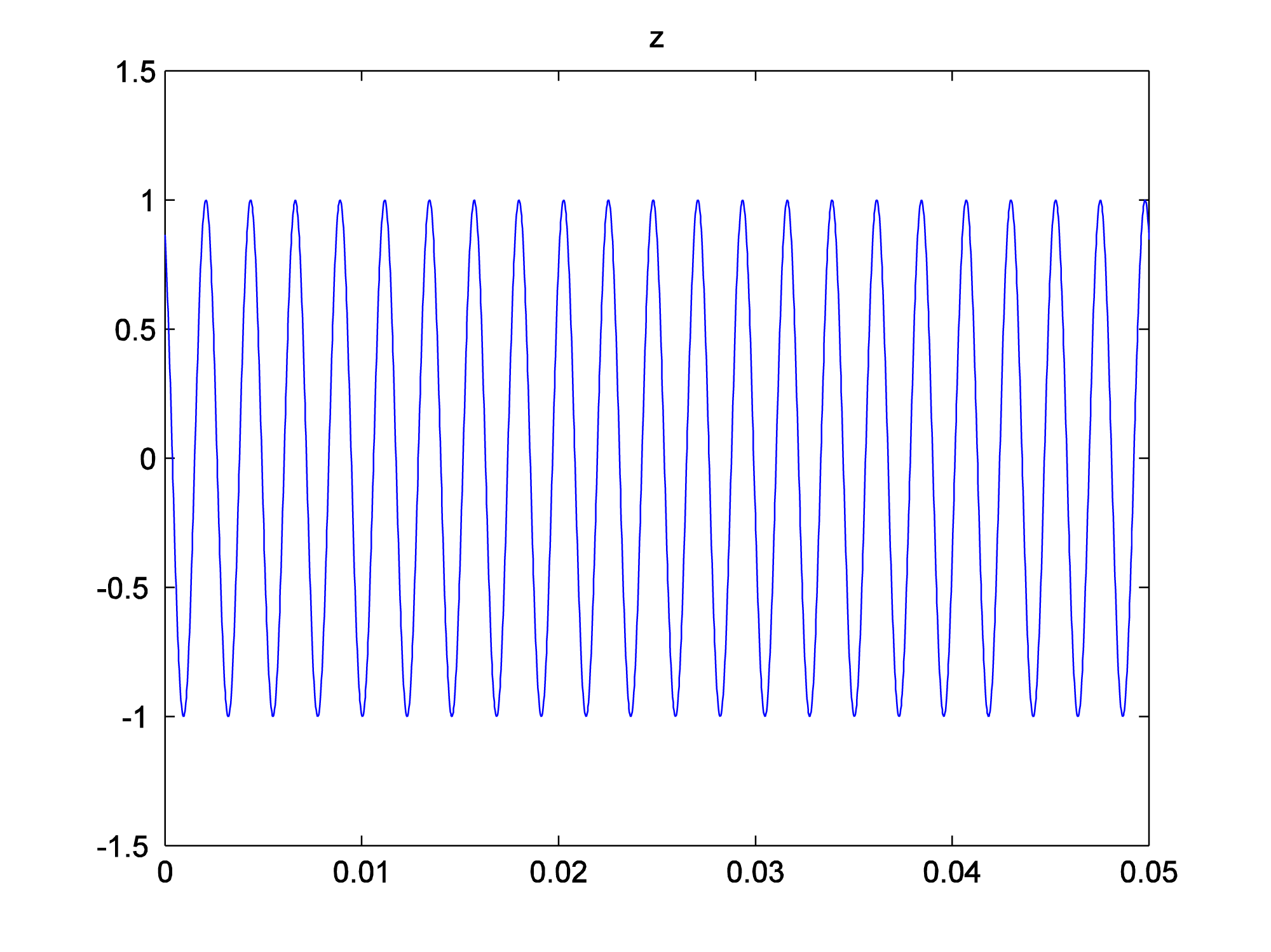
x = cos(2*pi*110*t);
y = cos(2*pi*220*t + pi/3);
z = cos(2*pi*440*t + pi/6);
x, y, and z are arrays of numbers that can be used as audio samples. pi/3 and pi/6 represent phase shifts for the 220 Hz and 440 Hz waves, to make our phase response graph more interesting. The figures can be displayed with the following:
figure;
plot(t,x);
axis([0 0.05 -1.5 1.5]);
title('x');
figure;
plot(t,y);
axis([0 0.05 -1.5 1.5]);
title('y');
figure;
plot(t,z);
axis([0 0.05 -1.5 1.5]);
title('z');
We look at only the first 0.05 seconds of the waveforms in order to see their shape better. You can see the phase shifts in the figures below. The second and third waves don’t start at 0 on the vertical axis.


Now we add the three sine waves to create a composite wave that has three frequency components at three different phases.
a = (x + y + z)/3;
Notice that we divide the summed sound waves by three so that the sound doesn’t clip. You can graph the three-component sound wave with the following:
figure;
plot(t, a);
axis([0 0.05 -1.5 1.5]);
title('a = x + y + z');
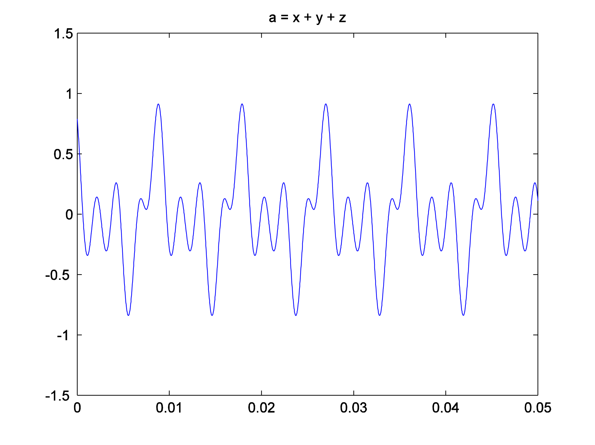
This is a graph of the sound wave in the time domain. You could call it an impulse response graph, although when you’re looking at a sound file like this, you usually just think of it as “sound data in the time domain.” The term “impulse response” is used more commonly for time domain filters, as we’ll see in Chapter 7. You might want to play the sound to be sure you have what you think you have. The sound function requires that you tell it the number of samples it should play per second, which for our simulation is 44,100.
sound(a, sr);
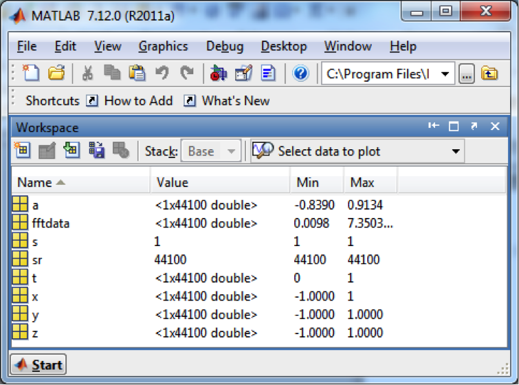
When you play the sound file and listen carefully, you can hear that it has three tones. MATLAB’s Fourier transform (fft) returns an array of double complex values (double-precision complex numbers) that represent the magnitudes and phases of the frequency components.
fftdata = fft(a);
In MATLAB’s workspace window, fftdata values are labeled as type double, giving the impression that they are real numbers, but this is not the case. In fact, the Fourier transform produces complex numbers, which you can verify by trying to plot them in MATLAB. The magnitudes of the complex numbers are given in the Min and Max fields, which is computed by the abs function. For a complex number $$a+bi$$, the magnitude is computed as $$\sqrt{a^{2}+b^{2}}$$. MATLAB does this computation and yields the magnitude.
To plot the results of the fft function such that the values represent the magnitudes of the frequency components, we first apply the abs function to fftdata.
fftmag = abs(fftdata);
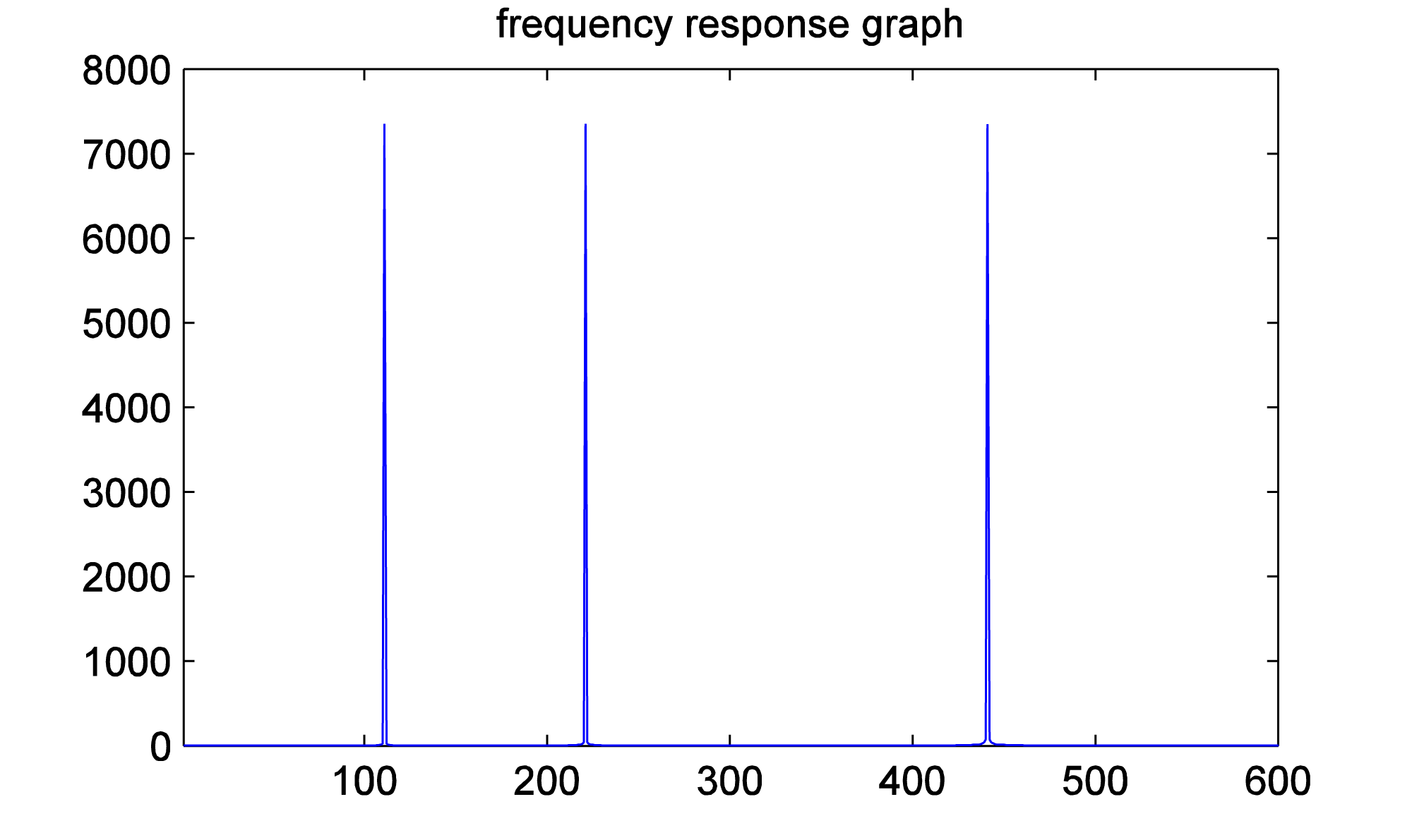
Let’s plot the frequency components to be sure we have what we think we have. For a sampling rate of sr on an array of sample values of size N, the Fourier transform returns the magnitudes of $$N/2$$ frequency components evenly spaced between 0 and sr/2 Hz. (We’ll explain this completely in Chapter 5.) Thus, we want to display frequencies between 0 and sr/2 on the horizontal axis, and only the first sr/2 values from the fftmag vector.
figure;
freqs = [0: (sr/2)-1];
plot(freqs, fftmag(1:sr/2));
[aside]If we would zoom in more closely at each of these spikes at frequencies 110, 220, and 440 Hz, we would see that they are not perfectly horizontal lines. The “imperfect” results of the FFT will be discussed later in the sections on FFT windows and windowing functions.[/aside] When you do this, you’ll see that all the frequency components are way over on the left side of the graph. Since we know our frequency components should be 110 Hz, 220 Hz, and 440 Hz, we might as well look at only the first, say, 600 frequency components so that we can see the results better. One way to zoom in on the frequency response graph is to use the zoom tool in the graph window, or you can reset the axis properties in the command window, as follows.
axis([0 600 0 8000]);
This yields the frequency response graph for our composite wave, which shows the three frequency components.
To get the phase response graph, we need to extract the phase information from the fftdata. This is done with the angle function. We leave that as an exercise. Let’s try the Fourier transform on a more complex sound wave – a sound file that we read in.
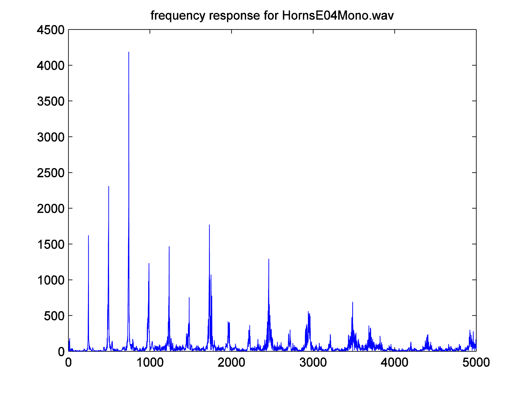
y = audioread('HornsE04Mono.wav');
As before, you can get the Fourier transform with the fft function.
fftdata = fft(y);
You can then get the magnitudes of the frequency components and generate a frequency response graph from this.
fftmag = abs(fftdata);
figure;
freqs = [0:(sr/2)-1];
plot(freqs, fftmag(1:sr/2));
axis([0 sr/2 0 4500]);
title('frequency response for HornsE04Mono.wav');
Let’s zoom in on frequencies up to 5000 Hz.
axis([0 5000 0 4500]);
The graph below is generated.
The inverse Fourier transform gives us back our original sound data in the time domain.
ynew = ifft(fftdata);
If you compare y with ynew, you’ll see that the inverse Fourier transform has recaptured the original sound data.
2.3.10 Windowing the FFT
When we applied the Fourier transform in MATLAB in Section 2.3.9, we didn’t specify a window size. Thus, we were applying the FFT to the entire piece of audio. If you listen to the WAV file HornsE04Mono.wav, a three second clip, you’ll first hear some low tubas and them some higher trumpets. Our graph of the FFT shows frequency components up to and beyond 5000 Hz, which reflects the sounds in the three seconds. What if we do the FFT on just the first second (44100 samples) of this WAV file, as follows? The resulting frequency components are shown in Figure 2.49.
y = audioread('HornsE04Mono.wav');
sr = 44100;
freqs = [0:(sr/2)-1];
ybegin = y(1:44100);
fftdata2 = fft(ybegin);
fftdata2 = fftdata2(1:22050);
plot(freqs, abs(fftdata2));
axis([0 5000 0 4500]);
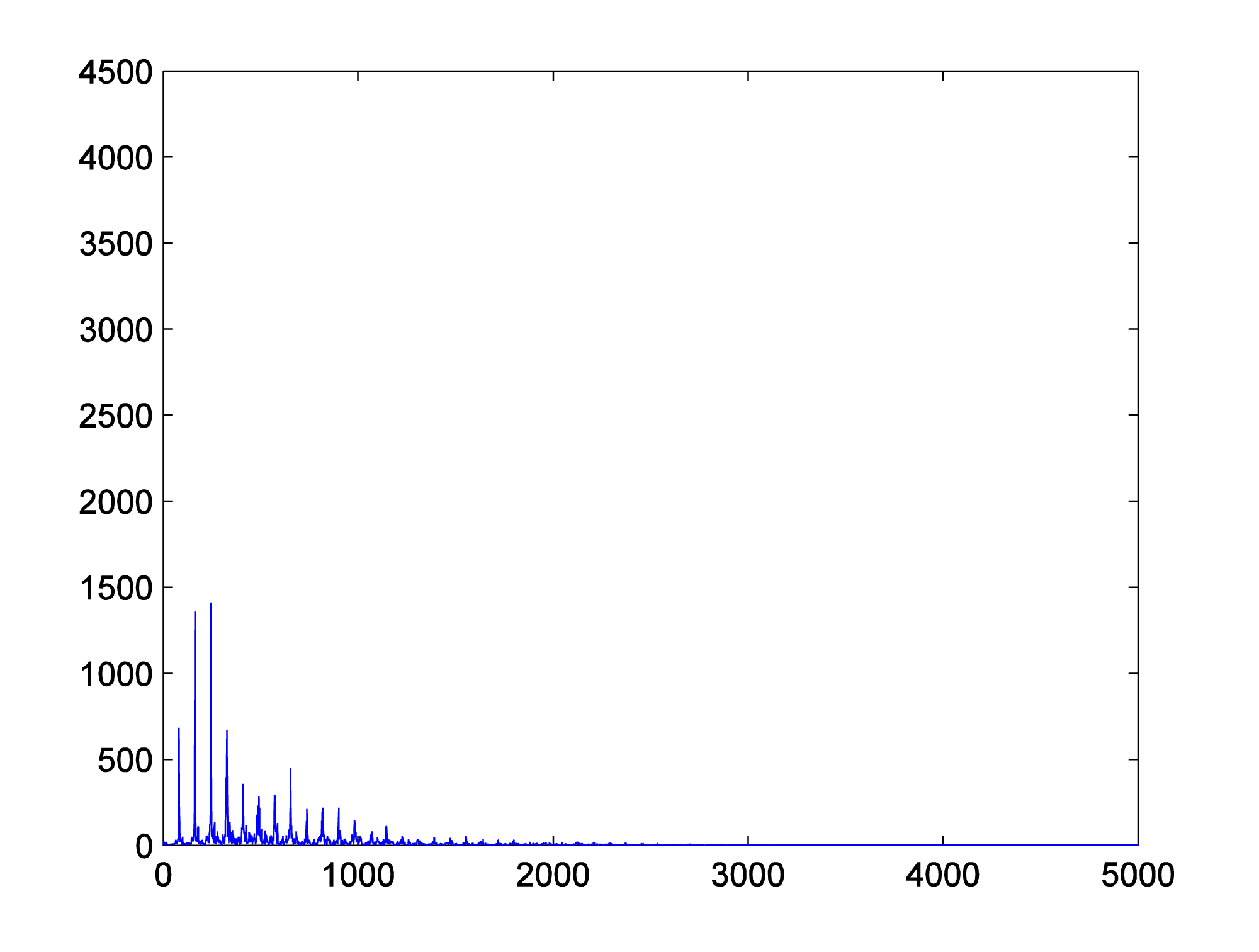
What we’ve done is focus on one short window of time in applying the FFT. An FFT window is a contiguous segment of audio samples on which the transform is applied. If you consider the nature of sound and music, you’ll understand why applying the transform to relatively small windows makes sense. In many of our examples in this book, we generate segments of sound that consist of one or more frequency components that do not change over time, like a single pitch note or a single chord being played without change. These sounds are good for experimenting with the mathematics of digital audio, but they aren’t representative of the music or sounds in our environment, in which the frequencies change constantly. The WAV file HornsE04Mono.wav serves as a good example. The clip is only three seconds long, but the first second is very different in frequencies (the pitches of tubas) from the last two seconds (the pitches of trumpets). When we do the FFT on the entire three seconds, we get a kind of “blurred” view of the frequency components, because the music actually changes over the three second period. It makes more sense to look at small segments of time. This is the purpose of the FFT window.
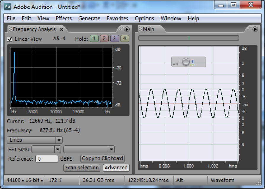
Figure 2.50 shows an example of how FFT window sizes are used in audio processing programs. Notice the drop down menu, which gives you a choice of FFT sizes ranging from 32 to 65536 samples. The FFT window size is typically a power of 2. If your sampling rate is 44,100 samples per second, then a window size of 32 samples is about 0.0007 s, and a window size of 65536 is about 1.486 s.
There’s a tradeoff in the choice of window size. A small window focuses on the frequencies present in the sound over a short period of time. However, as mentioned earlier, the number of frequency components yielded by an FFT of size N is N/2. Thus, for a window size of, say, 128, only 64 frequency bands are output, these bands spread over the frequencies from 0 Hz to sr/2 Hz where sr is the sampling rate. (See Chapter 5.) For a window size of 65536, 37768 frequency bands are output, which seems like a good thing, except that with the large window size, the FFT is not isolating a short moment of time. A window size of around 2048 usually gives good results. If you set the size to 2048 and play the piece of music loaded into Audition, you’ll see the frequencies in the frequency analysis view bounce up and down, reflecting the changing frequencies in the music as time pass.
