2.2.1 Acoustics
In each chapter, we begin with basic concepts in Section 1 and give applications of those concepts in Section 2. One main area where you can apply your understanding of sound waves is in the area of acoustics. “Acoustics” is a large topic, and thus we have devoted a whole chapter to it. Please refer to Chapter 4 for more on this topic.
2.2.2 Sound Synthesis
Naturally occurring sound waves almost always contain more than one frequency. The frequencies combined into one sound are called the sound’s frequency components. A sound that has multiple frequency components is a complex sound wave. All the frequency components taken together constitute a sound’s frequency spectrum. This is analogous to the way light is composed of a spectrum of colors. The frequency components of a sound are experienced by the listener as multiple pitches combined into one sound.
To understand frequency components of sound and how they might be manipulated, we can begin by synthesizing our own digital sound. Synthesis is a process of combining multiple elements to form something new. In sound synthesis, individual sound waves become one when their amplitude and frequency components interact and combine digitally, electrically, or acoustically. The most fundamental example of sound synthesis is when two sound waves travel through the same air space at the same time. Their amplitudes at each moment in time sum into a composite wave that contains the frequencies of both. Mathematically, this is a simple process of addition.
[wpfilebase tag=file id=29 tpl=supplement /]
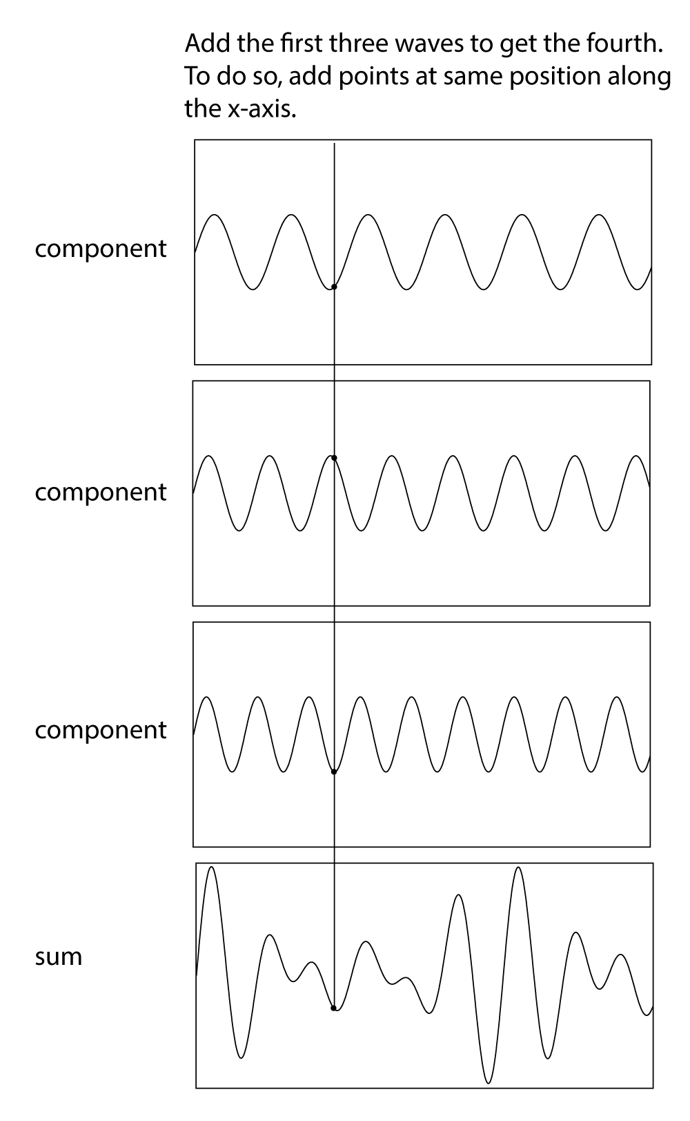
We can experiment with sound synthesis and understand it better by creating three single-frequency sounds using an audio editing program like Audacity or Adobe Audition. Using the “Generate Tone” feature in Audition, we’ve created three separate sound waves – the first at 262 Hz (middle C on a piano keyboard), the second at 330 Hz (the note E), and the third at 393 Hz (the note G). They’re shown in Figure 2.14, each on a separate track. The three waves can be mixed down in the editing software – that is, combined into a single sound wave that has all three frequency components. The mixed down wave is shown on the bottom track.
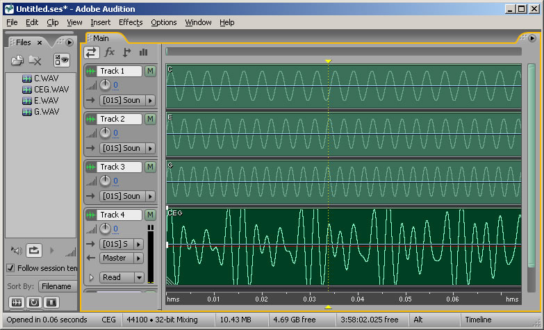
In a digital audio editing program like Audition, a sound wave is stored as a list of numbers, corresponding to the amplitude of the sound at each point in time. Thus, for the three audio tones generated, we have three lists of numbers. The mix-down procedure simply adds the corresponding values of the three waves at each point in time, as shown in Figure 2.15. Keep in mind that negative amplitudes (rarefactions) and positive amplitudes (compressions) can cancel each other out.
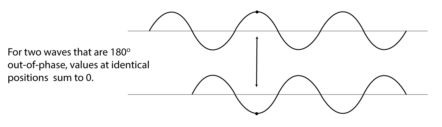
We’re able to hear multiple sounds simultaneously in our environment because sound waves can be added. Another interesting consequence of the addition of sound waves results from the fact that waves have phases. Consider two sound waves that have exactly the same frequency and amplitude, but the second wave arrives exactly one half cycle after the first – that is, 180o out-of-phase, as shown in Figure 2.16. This could happen because the second sound wave is coming from a more distant loudspeaker than the first. The different arrival times result in phase-cancellations as the two waves are summed when they reach the listener’s ear. In this case, the amplitudes are exactly opposite each other, so they sum to 0.
2.2.3 Sound Analysis
We showed in the previous section how we can add frequency components to create a complex sound wave. The reverse of the sound synthesis process is sound analysis, which is the determination of the frequency components in a complex sound wave. In the 1800s, Joseph Fourier developed the mathematics that forms the basis of frequency analysis. He proved that any periodic sinusoidal function, regardless of its complexity, can be formulated as a sum of frequency components. These frequency components consist of a fundamental frequency and the harmonic frequencies related to this fundamental. Fourier’s theorem says that no matter how complex a sound is, it’s possible to break it down into its component frequencies – that is, to determine the different frequencies that are in that sound, and how much of each frequency component there is.
[aside]”Frequency response” has a number of related usages in the realm of sound. It can refer to a graph showing the relative magnitudes of audible frequencies in a given sound. With regard to an audio filter, the frequency response shows how a filter boosts or attenuates the frequencies in the sound to which it is applied. With regard to loudspeakers, the frequency response is the way in which the loudspeakers boost or attenuate the audible frequencies. With regard to a microphone, the frequency response is the microphone’s sensitivity to frequencies over the audible spectrum.[/aside]
Fourier analysis begins with the fundamental frequency of the sound – the frequency of the longest repeated pattern of the sound. Then all the remaining frequency components that can be yielded by Fourier analysis – i.e., the harmonic frequencies – are integer multiples of the fundamental frequency. By “integer multiple” we mean that if the fundamental frequency is $$f_0$$ , then each harmonic frequency $$f_n$$ is equal to for some non-negative integer $$(n+1)f_0$$.
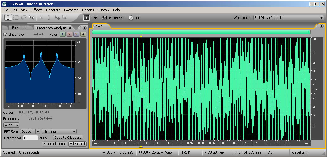
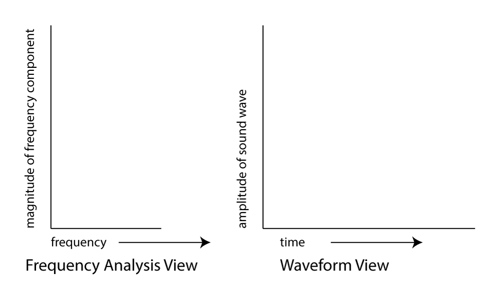
The Fourier transform is a mathematical operation used in digital filters and frequency analysis software to determine the frequency components of a sound. Figure 2.17 shows Adobe Audition’s waveform view and a frequency analysis view for a sound with frequency components at 262 Hz, 330 Hz, and 393 Hz. The frequency analysis view is to the left of the waveform view. The graph in the frequency analysis view is called a frequency response graph or simply a frequency response. The waveform view has time on the x-axis and amplitude on the y-axis. The frequency analysis view has frequency on the x-axis and the magnitude of the frequency component on the y-axis. (See Figure 2.18.) In the frequency analysis view in Figure 2.17, we zoomed in on the portion of the x-axis between about 100 and 500 Hz to show that there are three spikes there, at approximately the positions of the three frequency components. You might expect that there would be three perfect vertical lines at 262, 330, and 393 Hz, but this is because digitizing and transforming sound introduces some error. Still, the Fourier transform is accurate enough to be the basis for filters and special effects with sounds.
In the example just discussed, the frequencies that are combined in the composite sound never change. This is because of the way we constructed the sound, with three single-frequency waves that are held for one second. This sound, overall, is periodic because the pattern created from adding these three component frequencies is repeated over time, as you can see in the bottom of Figure 2.14.
Natural sounds, however, generally change in their frequency components as time passes. Consider something as simple as the word “information.” When you say “information,” your voice produces numerous frequency components, and these change over time. Figure 2.19 shows a recording and frequency analysis of the spoken word “information.”
When you look at the frequency analysis view, don’t be confused into thinking that the x-axis is time. The frequencies being analyzed are those that are present in the sound around the point in time marked by the yellow line.

In music and other sounds, pitches – i.e., frequencies – change as time passes. Natural sounds are not periodic in the way that a one-chord sound is. The frequency components in the first second of such sounds are different from the frequency components in the next second. The upshot of this fact is that for complex non-periodic sounds, you have to analyze frequencies over a specified time period, called a window. When you ask your sound analysis software to provide a frequency analysis, you have to set the window size. The window size in Adobe Audition’s frequency analysis view is called “FFT size.” In the examples above, the window size is set to 65536, indicating that the analysis is done over a span of 65,536 audio samples. The meaning of this window size is explained in more detail in Chapter 7. What is important to know at this point is that there’s a tradeoff between choosing a large window and a small one. A larger window gives higher resolution across the frequency spectrum – breaking down the spectrum into smaller bands – but the disadvantage is that it “blurs” its analysis of the constantly changing frequencies across a larger span of time. A smaller window focuses on what the frequency components are in a more precise, short frame of time, but it doesn’t yield as many frequency bands in its analysis.
2.2.4 Frequency Components of Non-Sinusoidal Waves
[wpfilebase tag=file id=108 tpl=supplement /]
In Section 2.1.3, we categorized waves by the relationship between the direction of the medium’s movement and the direction of the wave’s propagation. Another useful way to categorize waves is by their shape – square, sawtooth, and triangle, for example. These waves are easily described in mathematical terms and can be constructed artificially by adding certain harmonic frequency components in the right proportions. You may encounter square, sawtooth, and triangle waves in your work with software synthesizers. Although these waves are non-sinusoidal – i.e., they don’t take the shape of a perfect sine wave – they still can be manipulated and played as sound waves, and they’re useful in simulating the sounds of musical instruments.
A square wave rises and falls regularly between two levels (Figure 2.20, left). A sawtooth wave rises and falls at an angle, like the teeth of a saw (Figure 2.20, center). A triangle wave rises and falls in a slope in the shape of a triangle (Figure 2.20, right). Square waves create a hollow sound that can be adapted to resemble wind instruments. Sawtooth waves can be the basis for the synthesis of violin sounds. A triangle wave sounds very similar to a perfect sine wave, but with more body and depth, making it suitable for simulating a flute or trumpet. The suitability of these waves to simulate particular instruments varies according to the ways in which they are modulated and combined.

[aside]If you add the even numbered frequencies, you still get a sawtooth wave, but with double the frequency compared to the sawtooth wave with all frequency components.[/aside]
[wpfilebase tag=file id=11 tpl=supplement /]
Non-sinusoidal waves can be generated by computer-based tools – for example, Reason or Logic, which have built-in synthesizers for simulating musical instruments. Mathematically, non-sinusoidal waveforms are constructed by adding or subtracting harmonic frequencies in various patterns. A perfect square wave, for example, is formed by adding all the odd-numbered harmonics of a given fundamental frequency, with the amplitudes of these harmonics diminishing as their frequencies increase. The odd-numbered harmonics are those with frequency fn where f is the fundamental frequency and n is a positive odd integer. A sawtooth wave is formed by adding all harmonic frequencies related to a fundamental, with the amplitude of each frequency component diminishing as the frequency increases. If you would like to look at the mathematics of non-sinusoidal waves more closely, see Section 2.3.2.
[separator top=”1″ bottom=”0″ style=”none”]
2.2.5 Frequency, Impulse, and Phase Response Graphs
[aside]Although the term “impulse response” could technically be used for any instance of sound in the time domain, it is more often used to refer to instances of sound that are generated from a short burst of sound like a gun shot or balloon pop. In Chapter 7, you’ll see how an impulse response can be used to simulate the effect of an acoustical space on a sound.[/aside]
Section 2.2.3 introduces frequency response graphs, showing one taken from Adobe Audition. In fact, there are three interrelated graphs that are often used in sound analysis. Since these are used in this and later chapters, this is a good time to introduce you to these types of graphs. The three types of graphs are impulse response, frequency response, and phase response.
Impulse, frequency, and phase response graphs are simply different ways of storing and graphing the same set of data related to an instance of sound. Each type of graph represents the information in a different mathematical domain. The domains and ranges of the three types of sound graphs are given in Table 2.2.
[table caption=”Table 2.2 Domains and ranges of impulse, frequency, and phase response graphs” width=”80%”]
graph type,domain (x-axis),range (y-axis)
impulse response,time,amplitude of sound at each moment in time
frequency response,frequency,magnitude of frequency across the audible spectrum of sound
phase response,frequency,phase of frequency across the audible spectrum of sound
[/table]
Let’s look at an example of these three graphs, each associated with the same instance of sound. The graphs in the figures below were generated by sound analysis software called Fuzzmeasure Pro.
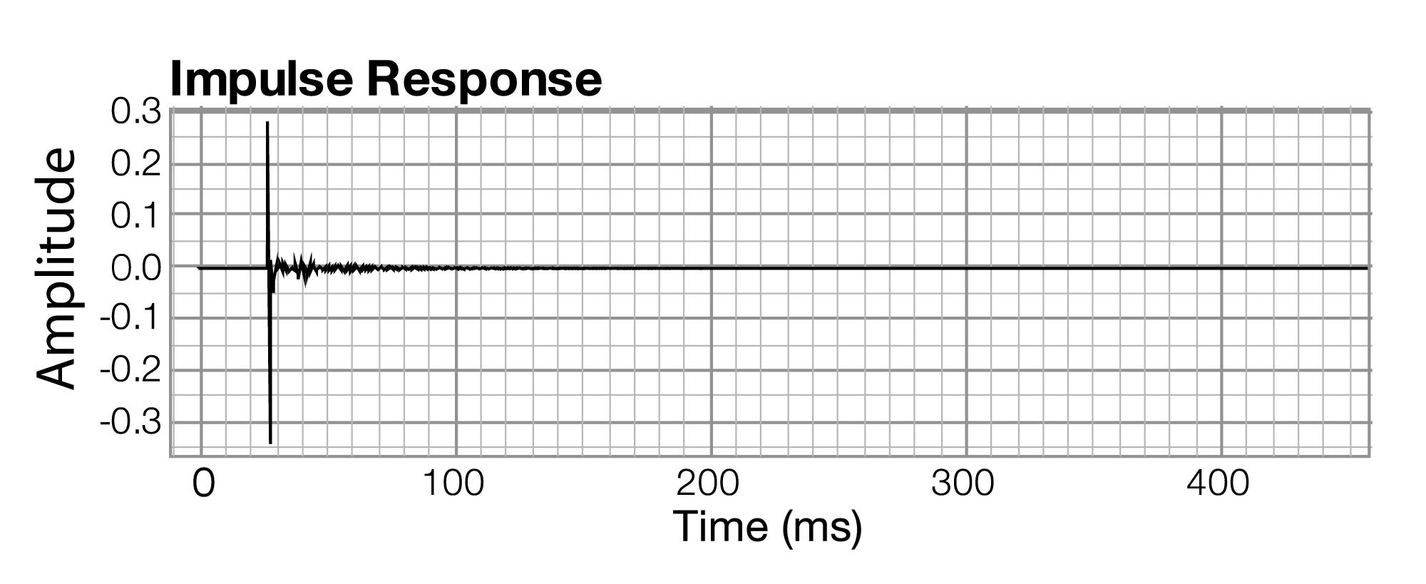

The impulse response graph shows the amplitude of the sound wave over time. The data used to draw this graph are produced by a microphone (and associated digitization hardware and software), which samples the amplitude of sound at evenly-spaced intervals of time. The details of this sound sampling process are discussed in Chapter 5. For now, all you need to understand is that when sound is captured and put into a form that can be handled by a computer, it is nothing more than a list of numbers, each number representing the amplitude of sound at a moment in time.
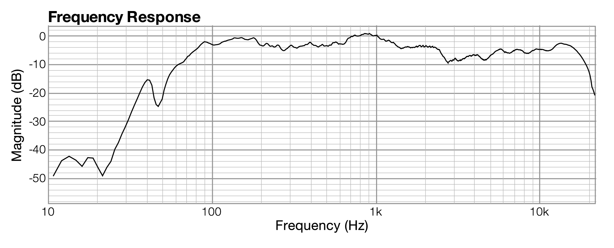
Related to each impulse response graph are two other graphs – a frequency response graph that shows “how much” of each frequency is present in the instance of sound, and a phase response graph that shows the phase that each frequency component is in. Each of these two graphs covers the audible spectrum. In Section 3, you’ll be introduced to the mathematical process – the Fourier transform – that converts sound data from the time domain to the frequency and phase domain. Applying a Fourier transform to impulse response data – i.e., amplitude represented in the time domain – yields both frequency and phase information from which you can generate a frequency response graph and a phase response graph. The frequency response graph has the magnitude of the frequency on the y-axis on whatever scale is chosen for the graph. The phase response graph has phases ranging from -180° to 180° on the y-axis.
The main points to understand are these:
- A graph is a visualization of data.
- For any given instance of sound, you can analyze the data in terms of time, frequency, or phase, and you can graph the corresponding data.
- These different ways of representing sound – as amplitude of sound over time or as frequency and phase over the audible spectrum – contain essentially the same information.
- The Fourier transform can be used to transform the sound data from one domain of representation to another. The Fourier transform is the basis for processes applied at the user-level in sound measuring and editing software.
- When you work with sound, you look at it and edit it in whatever domain of representation is most appropriate for your purposes at the time. You’ll see this later in examples concerning frequency analysis of live performance spaces, room modes, precedence effect, and so forth.
2.2.6 Ear Testing and Training
[wpfilebase tag=file id=31 tpl=supplement /]
If you plan to work in sound, it’s important to know the acuity of your own ears in three areas – the range of frequencies that you’re able to hear, the differences in frequencies that you can detect, and the sensitivity of your hearing to relative time and direction of sounds. A good place to begin is to have your hearing tested by an audiologist to discover the natural frequency response of your ears. If you want to do your own test, you can use a sine wave generator in Logic, Audition, or similar software to step through the range of audible sound frequencies and determine the lowest and highest ones you can hear. The range of human hearing is about 20 Hz to 20,000 Hz, but this varies with individuals and changes as an individual ages.
Not only can you test your ears for their current sensitivity; you also can train your ears to get better at identifying frequency and time differences in sound. Training your ears to recognize frequencies can be done by having someone boost frequency bands, one at a time, in a full-range noise or music signal while you guess which frequency is being boosted. In time, you’ll start “guessing” correctly. Training your ears to recognize time or direction differences requires that someone create two sound waves with location or time offsets and then ask you to discriminate between the two. The ability to identify frequencies and hear subtle differences is very valuable when working with sound. The learning supplements for this section give sample exercises and worksheets related to ear training.