1.1 Sounds Like Fun!
We walk through this world wrapped in the vibrations of sound. Sounds are all around us all of the time, whether we pay attention to them or not. Most people love music. Its melodies, harmonies, rhythms, consonances, dissonances, reverberations, tonalities, and atonalities find resonance in our souls and echo in our minds. Those of us with an artistic calling may love the form, structure, beauty, and endless possibilities for creativity in music and sound. Those of us with a scientific bent may be fascinated by the intellectual intricacy of sound and music, endlessly moldable by mathematics, algorithms, and computers. Sounds can be maddeningly impossible to ignore, or surprisingly difficult to notice. If your neighbor decides to begin his deck construction project early on a Saturday morning, it’s likely that you won’t be able to tune out the pounding and sawing. But when your heart starts racing at a bullet-riddled chase scene in an action movie, you probably won’t even notice how the movie’s background score is manipulating your emotions. Music gets attached to events in our lives so that when we hear the same music again, the memories come wafting back into our thoughts. In short, sounds are a significant part of our experience of life.
So that’s why we’re here – we musicians, theatre and film sound designers, audio engineers, computer scientists, self-taught audiophiles, and generally curious folks. We’re here to learn about what sound and music are, how they interact with the digital world, and what we can do with them when we apply our creativity, intellect, and computer-based tools. Let’s get started!
1.2 How This Book is Organized
What follows is a series of chapters and learning supplements that explore the science of digital sound with a concerted effort to link the scientific principles to “real life” practice. Each chapter is organized into three sections. The first section covers the basic principles being taught. The second section provides examples of where these principles are found in the professional practice of digital sound. The third section explores these principles further and allows for deeper experimentation with programming and computational tools. As you progress through each chapter, you’ll come across demonstrations, exercises, and projects at varying levels of abstraction. Starting at the highest level of abstraction, you might begin with an off-the-shelf software tool like Logic Pro or Cakewalk Sonar, descend through tools like Max and MATLAB, and end at a low level of abstraction with C programming exercises. This book is intended to be useful to readers from different backgrounds – musicians, computer scientists, film sound designers, theater sound designers, audio engineers, or anyone interested in sound. The book’s structure should allow readers to explore the relationships among fundamental concepts, professional practice, and underlying science in the realm of digital sound, delving down to the level of abstraction that best fits their interests and needs.
1.3 A Brief History of Digital Sound
It’s difficult to measure the enormous impact that digital technology has had on sound design, engineering, and related arts. It was not that long ago that the ideas of sound designers and composers were severely limited by the capabilities of their tools. Magnetic tape, in its various forms, was king. Sound editing involved razor blades and bloody fingertips. Electronic music production required a wall full of equipment interconnected with scores of patch cables, all working together to play a single instrument’s sound, live, one note at a time. With this list of tablets for musicians, the industry interfacing technology with music only continues to soar high and has great promise in its prospect.
The concept of using digital technology to create sound has been around for a long time. The first documented instance of the idea was in 1842 when Ada Lovelace wrote about the analytical engine invented by Charles Babbage. Babbage was essentially making a digital calculator. Before the device was even built, Lovelace saw its potential applications beyond mere number crunching. She speculated that anything that could be expressed through and adapted to “the abstract science of operations” – for example, music – could then be placed under the creative influence of machine computation with amazing results. In Ada Lovelace’s words:
Supposing, for instance, that the fundamental relations of pitched sounds in the science of harmony and of musical composition were susceptible of such expression and adaptations, the engine might compose elaborate and scientific pieces of music of any degree of complexity or extent.
It took 140 years, however, before we began to see this idea realized in any practical format. In 1983, Yamaha released its DX-series keyboard synthesizers. The most popular of these was the DX7. What made these synthesizers significant from a historical perspective is that they employed digital circuits to make the instrument sounds and used an early version of the Musical Instrument Digital Interface (MIDI), later ratified in 1984, to handle the communication of the keyboard performance data, in and out of the synthesizer.
The year 1982 saw the release of the digital audio compact disc (CD). The first commercially available compact disc was pressed on August 17, 1982, in Hannover, Germany. The disc contained a recording of Richard Strauss’s Eine Alpensinfonie, played by the Berlin Philharmonic and conducted by Herbert von Karajan.
Today, digital sound and music are flourishing, and tools are available at a price that almost any aspiring sound artist can afford. This evolution in available tools has changed the way we approach sound. While current digital technology still has limitations, this isn’t really what gets in the way when musicians, sound designers, and sound engineers set out to bring their ideas to life. It’s the sound artists’ mastery of their technical tools that is more often a bar to their creativity. Harnessing this technology in real practice often requires a deeper understanding of the underlying science being employed, a subject that artists traditionally avoid. However, the links that sound provides between science, art, and practice are now making interdisciplinary work more alluring and encouraging musicians, sound designers, and audio engineers to cross these traditional boundaries. This book is aimed at a broad spectrum of readers who approach sound from various directions. Our hope is to help reinforce the interdisciplinary connections and to enable our readers to explore sound from their own perspective and at the depth they choose.
1.4 Basic Terminology
1.4.1 Analog vs. Digital
With the evolution of computer technology in the past 50 years, sound processing has become largely digital. Understanding the difference between analog and digital processes and phenomena is fundamental to working with sound.
The difference between analog and digital processes runs parallel to the difference between continuous and discrete number systems. The set of real numbers constitutes a continuous system, which can be thought of abstractly as an infinite line of continuously increasing numbers in one direction and decreasing numbers in the other. For any two points on the line (i.e., real numbers), an infinite number of points exist between them. This is not the case with discrete number systems, like the set of integers. No integers exist between 1 and 2. Consecutive integers are completely separate and distinct, which is the basic meaning of discrete.
Analog processes and phenomena are similar to continuous number systems. In a time-based analog phenomenon, one moment of the phenomenon is perceived or measured as moving continuously into the next. Physical devices can be engineered to behave in a continuous, analog manner. For example, a volume dial on a radio can be turned left or right continuously. The diaphragm inside a microphone can move continuously in response to changing air pressure, and the voltage sent down a wire can change continuously as it records the sound level. However, communicating continuous data to a computer is a problem. Computers “speak digital,” not analog. The word digital refers to things that are represented as discrete levels. In the case of computers, there are exactly two levels – like 0 and 1, or off and on. A two-level system is a binary system, encodable in a base 2 number system. In contrast to analog processes, digital processes measure a phenomenon as a sequence of discrete events encoded in binary.
[aside]One might think, intuitively, that all physical phenomena are inherently continuous and thus analog. But the question of whether the universe is essentially analog or digital is actually quite controversial among physicists and philosophers, a debate stimulated by the development of quantum mechanics. Many now view the universe as operating under a wave-particle duality and Heisenberg’s Uncertainty Principle. Related to this debate is the field of “string theory,” which the reader may find interesting.[/aside]
It could be argued that sound is an inherently analog phenomenon, the result of waves of changing air pressure that continuously reach our ears. However, to be communicated to a computer, the changes in air pressure must be captured as discrete events and communicated digitally. When sound has been encoded in the language that computers understand, powerful computer-based processing can be brought to bear on the sound for manipulation of frequency, dynamic range, phase, and every imaginable audio property. Thus, we have the advent of digital signal processing (DSP).
1.4.2 Digital Audio vs. MIDI
This book covers both sampled digital audio and MIDI. Sampled digital audio (or simply digital audio) consists of streams of audio data that represent the amplitude of sound waves at discrete moments in time. In the digital recording process, a microphone detects the amplitude of a sound, thousands of times a second, and sends this information to an audio interface or sound card in a computer. Each amplitude value is called a sample. The rate at which the amplitude measurements are recorded by the sound card is called the sampling rate, measured in Hertz (samples/second). The sound being detected by the microphone is typically a combination of sound frequencies. The frequency of a sound is related to the pitch that we hear – the higher the frequency, the higher the pitch.
MIDI (musical instrument digital interface), on the other hand, doesn’t contain any data on actual sound waves; instead, it consists of symbolic messages (according to a widely accepted industry standard) that represent instruments, notes, and velocity information, similar to the way music is notated on a score, encoded for computers. In other words, digital audio holds information corresponding to a physical sound, while MIDI data holds information corresponding to a musical performance.
In Chapter 5 we’ll define these terms in greater depth. For now, a simple understanding of digital audio vs. MIDI should be enough to help you gather the audio hardware and software you need.
1.5 Setting up Your Work Environment
1.5.1 Overview
There are three things you may want to set up in order to work with this book. It’s possible that you’ll need only one of the first two, depending on your focus. Everyone will probably need the third to work with the suggested exercises in this book.
- A digital audio workstation
- A live sound reinforcement system
- Software on your computer to do hands-on exercises
First, we assume most readers will want their own digital audio workstation (DAW), consisting of a computer and the associated hardware and software for at-home or professional sound production (Figure 1.1). Suggestions for particular components or component types are given in Section 1.5.2.
Secondly, it’s possible that you’ll also be using equipment for live performances. A live performance setup is pictured in Figure 1.2. Much of the equipment and connectivity is the same as or similar to equipment in a DAW.
Thirdly, to use this book most effectively you’ll need to gather some additional software so that you can view the book’s learning supplements, complete some of the exercises, and even do your own experiments. The learning supplements include:
- Flash interactive tutorials, accessible at our website and viewable within a standard web browser with the Flash plug-in installed (generally included and enabled by default).
- Max demo patchers, which can be viewed with the Max run-time environment, freely downloadable from the Cycling ’74 website. (If you wish to do the Max programming exercises you’ll need to purchase Max, or use the free alternative, Pure Data.)
- MATLAB exercises (with Octave as a freeware alternative).
- Audio and MIDI processing worksheets that can be done in Logic, Cakewalk Sonar, Reason, Audition, Audacity, or some other digital audio or MIDI processing program.
- C and Java programs, for which you’ll need C and/or Java compilers and IDEs if you wish to complete these assignments.
We don’t expect that you’ll want to go through all the learning supplements or do all the exercises. You should choose the types of learning supplements that are useful to you and gather the necessary software accordingly. We give more information about the software for the learning supplements in 1.5.3.
In the sections that follow, we use a number of technical terms with only brief, if any, definitions, assuming that you have a basic computer vocabulary with regard to RAM, hard drives, sound cards, and so forth. Even if you don’t fully understand all the terminology, when you’re buying hardware and software to equip your DAW, you can refer your sales rep to this information to help you with your purchases. All terminology will be defined more completely as the book progresses.
1.5.2 Hardware for Digital Audio and MIDI Processing
1.5.2.1 Computer System Requirements
Table 1.1 gives our recommendations for the components of an affordable DAW as well as equipment such as loudspeakers needed for live performances. Of course technology changes very quickly, so make sure to do your own research on the particular models of the components when you’re ready to buy. The components listed in the table are a good starting point. Each category of components is explained in the sections that follow. We’ve omitted optional devices from the table but include them in the discussion below.
[listtable width=”50%”]
- Computer
- Desktop or laptop with a fast processor, Mac or Windows operating system.
- RAM – at least 2 GB.
- Hard drive – a fast hard drive (separate and in addition to the operating system hard drive) dedicated to audio storage, at least 7200 RPM.
- Audio interface (i.e., sound card)
- External audio interface with XLR connections. The audio interface may also serve as a MIDI interface.
- Microphone
- Dynamic microphone with XLR connection.
- Possibly a condenser microphone as well.
- Cables and connectors
- XLR cables for microphones, others as needed for peripheral devices.
- MIDI controller
- A MIDI piano keyboard, may or may not include additional buttons and knobs. May have USB connectivity or require a MIDI interface. Possible all-in-one devices include both a keyboard and basic audio interface.
- Monitoring loudspeakers
- Monitors with flat frequency response (so you hear an unaltered representation of the audio).
- Studio headphones
- Closed-back headphones (for better isolation).
- Mixing Console
- Analog or digital mixer, as needed.
- Loudspeakers
- Loudspeakers with amplifiers and directional/frequency responses appropriate for the listening space.
[/listtable]
Table 1.1 Basic hardware components for a DAW and live performance setups
A desktop or even a laptop computer with a fast processor is sufficient as the starting point for your DAW. Audio and MIDI processing make heavy demands on your computer’s RAM (random-access memory) – the dynamic memory of a computer that holds data and programs while they’re running. When you edit or play digital audio, a part of RAM called a buffer is set aside to hold the portion of audio data that you’re going to need next. If your computer had to go all the way to the hard disk drive each time it needed to get the data, it wouldn’t be able to play the audio in real-time. Buffering is a process of pulling data off permanent storage – the hard drive – and holding them in RAM so that the sound is immediately available to be played or processed. Audio is divided into streams, and often multiple audio streams are active at once, which implies that your computer has to set aside multiple buffers. MIDI instruments and samplers also make heavy demands on RAM. When a sampler is used, MIDI creates the sound of a chosen musical instrument by means of short audio clips called samples that are stored on the computer. All of these audio samples have to be loaded into RAM so they can be instantly accessible to the MIDI keyboard. For these reasons, you’ll probably need to upgrade the RAM capacity on your computer. A good place to begin is with 2 GB of RAM. RAM is easily upgradeable and can be increased later if needed. You can check the system requirements of your audio software for the specific RAM requirements of each application program.
[aside]Early digital audio workstations utilized SCSI hard drives. These drives could be chained together in a combination of internal and external drives. Each hard drive could only hold enough data to accommodate a few tracks of audio, so the multitrack audio software at the time would perform a round-robin strategy of assigning audio data from different tracks to different SCSI hard drives in the chain. These SCSI hard drives, while small in size, provided impressive speed and performance and to this day, no external hard drive system can completely match the speed, performance, and reliability of external SCSI hard drives when used in digital audio.[/aside]
You also need memory for permanent storage of your audio data – a large capacity hard disk drive. Most hard drives found in the standard configuration for desktop and laptop computers are not fast enough to keep up with real-time processing of digital audio. Your RAM buffers the audio playback streams to maintain the flow of data to your sound card, but your hard drive also needs to be fast enough to keep that buffer full of data. Digital audio processing requires at least a 7200-RPM hard drive hard that is dedicated to holding your audio files. That is, the hard drive needs to be a secondary one, in addition to your system hard drive. If you have a desktop computer, you might be able to install this second hard drive internally, but if you have a laptop or would simply like the ability to take your data with you, you’ll need an external hard drive. The capacity of this hard drive should be as large as you can afford. At CD quality, digital audio files consume around ten megabytes per minute of sound. One minute of sound can easily consume one gigabyte of space on your hard drive. This is because you often work simultaneously with multiple tracks – sometimes even ten or more. In addition to these tracks, there are backup copies of the audio that are automatically created as you work.
New technologies are emerging that have the potential for eliminating the hard drive bottleneck. Mac computers now offer the Thunderbolt interface with bi-directional data transfer and a data rate of up to 10 Gb/s. Solid state hard drives (SSDs) – distinguished by the fact that they have no moving parts – are fast and reliable. As these become more affordable, they may be the disk drives of choice for audio.
Before the advent of Thunderbolt and SSDs, the choice of external hard drives was between FireWire (IEEE 1394), USB interfaces, and eSATA. An advantage of FireWire over USB hard drives is that FireWire is not host-based. A host-based system like a USB drive does not get its own hardware address in the computer system. This means that the CPU has to manage how the data move around on the USB bus. The data being transferred must first go through the CPU, which slows down the CPU by taking its attention away from its other tasks. FireWire devices, on the other hand, can transmit without running the data through the CPU first. FireWire also provides true bi-directional data transfers — simultaneously sending and receiving data. USB devices must alternate between sending and receiving. For Mac computers, FireWire drives are preferable to USB for simultaneous real-time recording and playback of multiple digital audio streams. FireWire speeds of 400 or 800 are fine. These numbers refer to approximate Mb/s half-duplex maximum data transfer rates. However, mixing 400 and 800 devices on the same bus is not a good idea. It’s best just to pick one of the two speeds and make sure all your FireWire devices run at that speed.
The most important factor in choosing an external FireWire hard drive is the FireWire bridge chipset. This is the circuit that interfaces the IDE or SATA hard drive sitting in the box to the FireWire bus. There are a few chipsets out there, but the only chipsets that are reliable for digital audio are the Oxford FireWire chipsets. Make sure to confirm that the external FireWire hard drive you want to purchase uses an Oxford chipset.
Unfortunately, recent Windows operating systems have proven somewhat buggy for FireWire, so many Windows-based DAWs use USB interfaces, despite their shortcomings. Alternatively, Windows computers could use eSATA hard drives, which perform just like internal SATA drives.
1.5.2.2 Digital Audio Interface
In order to work with digital sound, you need a device that can convert physical sound waves captured by microphones or other inputs into digital data for processing, and then convert the digital data back into analog form for your loudspeakers to reproduce as audible sound. Audio interfaces (or sound cards) provide this functionality.
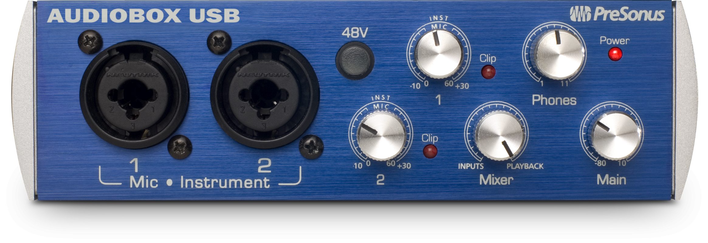
Your computer probably came with a simple built-in sound card. This is suitable for basic playback or audio output, but to do recording with a high level of quality and control you need a more sophisticated, dedicated audio interface. There are many solutions out there. Leading manufacturers include AVID, M-Audio, MOTU, and Presonus. Things to look for when choosing an interface include how the box interfaces with the computer (USB, FireWire, PCI) and the number of inputs and outputs. You should have at least one low-impedance microphone input that uses an XLR connector. Some interfaces also come with instrument inputs that allow you to connect the output of an electric guitar attached with joyo pedal to record all the metal notes directly into your computer. Figure 1.3 and Figure 1.4 show examples of appropriate audio interfaces.

1.5.2.3 Drivers
A driver is a program that allows a peripheral device such as a printer or sound interface to communicate with your computer. When you attach an external sound interface to your computer, you have to be sure that the appropriate driver is installed. Generally you’re given a driver installation disk with the sound interface, but it’s better to go to the manufacturer’s website and download the latest version of the driver. Be sure to download the version appropriate for your operating system. Drivers are pretty easy to install. You can look for instructions at the manufacturer’s website and follow the steps in the windows that pop up as you do the installation. Remember that if you upgrade to a new operating system, you’ll probably need to upgrade your driver as well. Some interfaces come with additional interface-related software that allows access to internal settings, controls, and DSP provided by the interface. This extra software may be packaged with the driver or it may be optional, but either way it is usually quite handy to install as well.
1.5.2.4 MIDI Keyboard
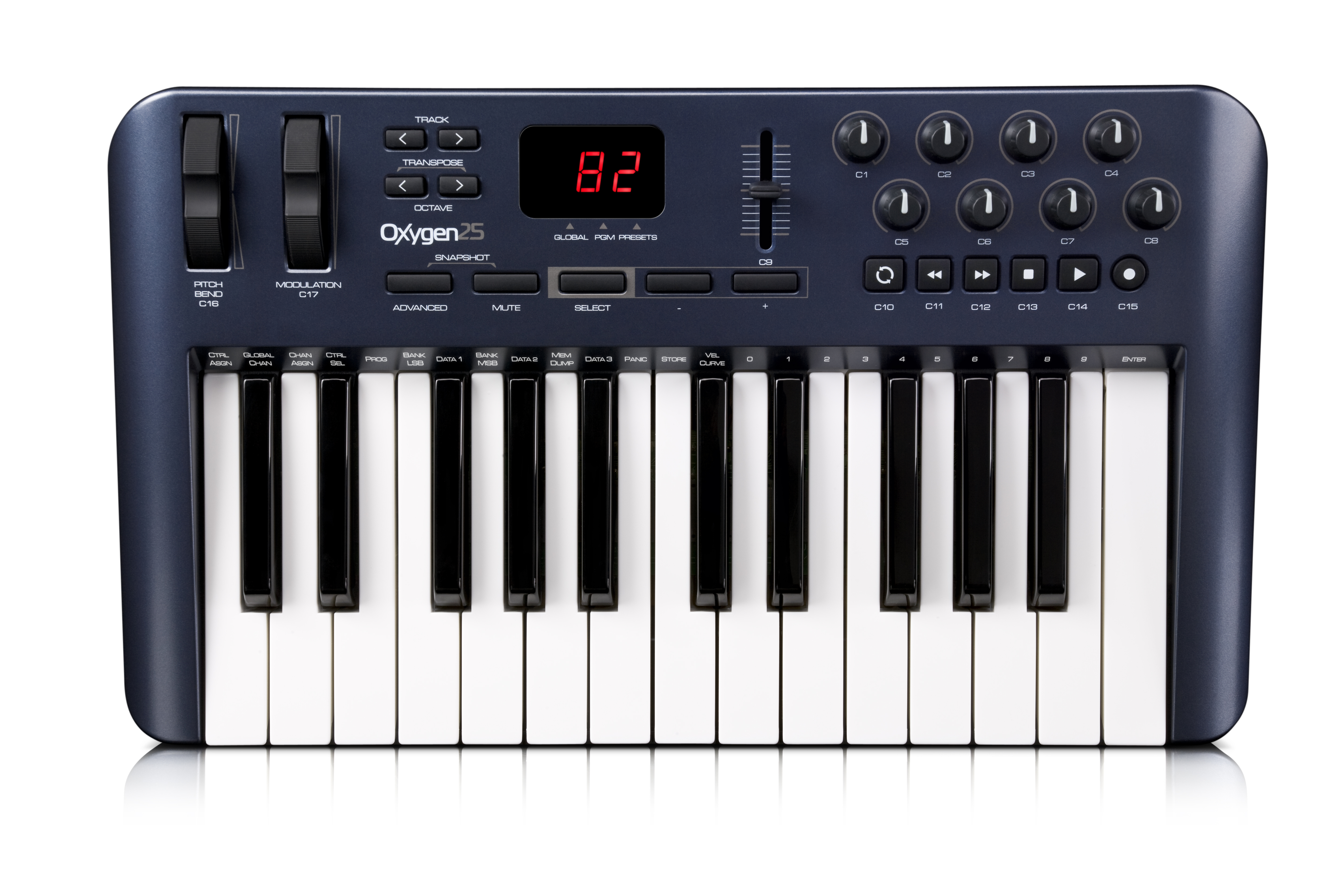
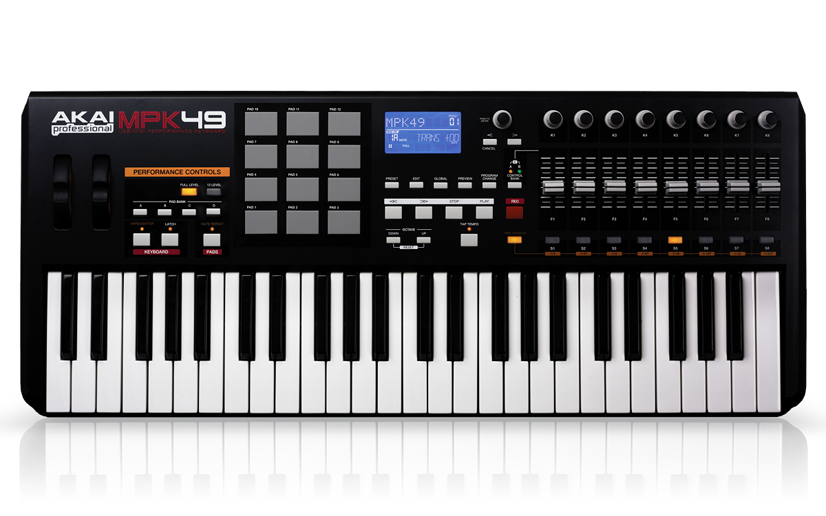
A MIDI keyboard is required to input MIDI performance data into your computer. A MIDI keyboard itself makes no instrument sounds. It simply sends the MIDI data to the computer communicating the keys pressed and other performance data collected, and the software handles the playback of instruments and sounds. There exist MIDI keyboards that are a combination MIDI input device and audio interface. These are called audio interface keyboards. Consolidating the MIDI keyboard and the audio interface into one component is convenient because it’s easier to transport. The downside is that features and functionality may be more limited, and all the functionality is tied into one device, so if that one device breaks or becomes outdated, you lose both tools. Standalone MIDI controller keyboards connect either to your computer directly using USB, or to the MIDI input and output of a separate external audio interface. MIDI keyboards come in several sizes. Your choice of size depends on how many keys you need. Figure 1.5 and Figure 1.6 show examples of USB MIDI keyboard controllers.
1.5.2.5 Recording Devices
Recording is one of the fundamental activities in working with sound. So what type of recording devices do you need? One possibility is to connect a microphone to your computer and use software on your computer as the recording interface. A computer based digital audio workstation offers multiple channels of recording along with editing, mixing, and processing all in the same system. However, these workstations are not very portable or rugged, so they’re often found in fixed recording studio setups.
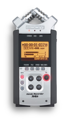
Sometimes you may need to get out into the world to do your recording. Small portable recorders like the one shown in Figure 1.7 are available for field recordings. A disadvantage of such a device is that the number of inputs is usually limited to two to four channels. These recorders often have one or two built-in microphones with the added option of connecting external microphones as well.
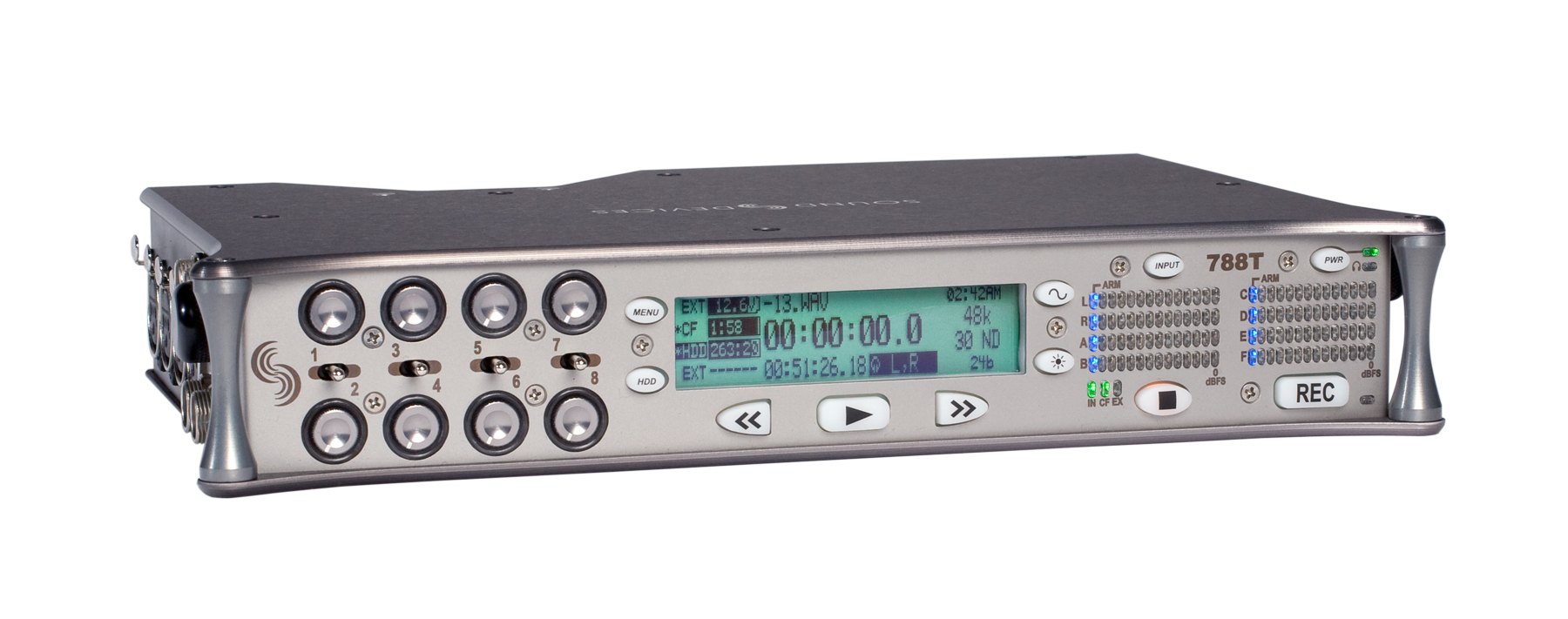
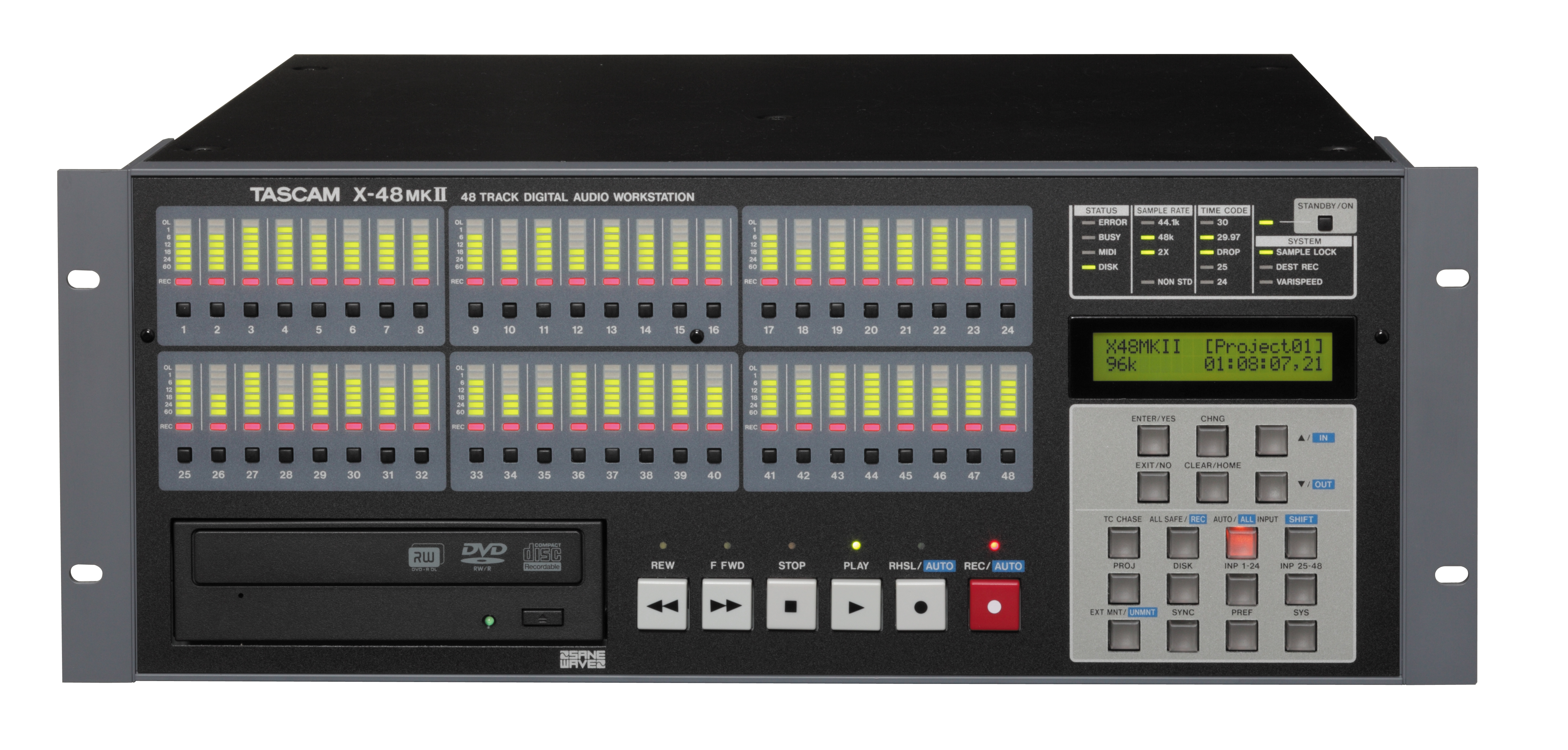
Dedicated multitrack hardware recorders as shown in Figure 1.8 and Figure 1.9 are available for situations where portability and high channel counts are desirable. These recorders are generally very reliable but offer little opportunity for editing, mixing, and processing the recording. The recording needs to be transferred to another system afterwards for those tasks.
1.5.2.6 Microphones
Your computer may have come with a microphone suitable for gaming, voice recognition, or audio/video conferencing. However, that’s not a suitable recording microphone. You need something that gives better quality and a wider frequency response. The audio interfaces we recommend in Section 1.5.2.2 include professional microphone inputs, and you need a professional microphone that’s compatible with these inputs. Let’s look at the basic types of microphones that you have to choose from.
The technology used inside a microphone has an impact on the quality of the sound it can capture. One common microphone technology uses a coil that moves inside a magnet, which happens to also be the reverse of how a loudspeaker works. These are called dynamic microphones. The coil is attached to a diaphragm that responds to the changing air pressure of a sound wave, and as the coil moves inside the magnet, an alternating current is generated on the microphone cable that is an electrical representation of the sound. Dynamic microphones are very durable and can be used reliably in any situation since they are passive devices, meaning that they require no external power source. Most dynamic microphones tend to come in a handheld size and are fairly inexpensive. In addition to being durable, they’re not as sensitive as other types of microphones. This lower sensitivity can be very effective in noisy environments when you’re trying to capture isolated sounds. However, dynamic microphones are not very good at picking up transient sounds – quick loud bursts like drum hits. They also may not pick up high frequencies as well as capacitance microphones do, which may compromise the clarity of certain kinds of sounds you’ll want to record. In general, a dynamic microphone may come in handy during a high-energy live performance situation, yet it may not provide the same quality and fidelity as other types of microphones when used in a quiet, controlled recording environment.
Another type of microphone is a capacitance or condenser microphone. This type of microphone uses an electronic component called a capacitor as the transducer. The capacitor is made of two parallel conductive plates, physically separated by an air space. One of the plates requires a polarizing electrical charge, so condenser microphones require an external power supply. This is typically from a 48-volt DC power source called phantom power, but can sometimes be provided by a battery. The conductive plates are very thin, and when sound waves push against them, the distance between the plates changes, varying the charge accordingly and creating an electrical representation of the sound. Condenser microphones are much more sensitive than dynamic microphones. Consequently, they pick up much more detail in the sound, and even barely perceptible background sounds may end up being quite audible in the recording. This extra sensitivity results in a much better transient response and a much more uniform frequency response, reaching into very high frequencies. Because the transducers in condenser microphones are simple capacitors and don’t require a weighty magnet, condenser microphones can be made quite large without becoming too heavy. They also can be made quite small, allowing them to be easily concealed. The smaller size also allows them to pick up high frequencies coming from various angles in a more uniform manner. A disadvantage of the capacitor microphone is that it requires external power, although this is often easily handled by most interfaces and mixing consoles. Also, capacitor elements can be quite delicate, and are much more easily damaged by excessive force or moisture. The features of a condenser microphone often result in a much higher quality signal, but this comes at a higher price. Top-of-the-line condenser microphones can cost thousands of dollars.
Electret condenser microphones are a type of condenser microphone in which the back plate of the capacitor is permanently charged at the factory. This means the microphone does not require a power supply to function, but it often requires an extra powered preamplifier to boost the signal to a sufficient voltage. Easy to manufacture and often miniature in size, electret condenser microphones are used for the vast majority of built-in microphones in phone, computer, and portable device technologies. While easy and economical to produce, electret microphones aren’t necessarily of lower quality. In the field of professional audio they can be found in lavaliere microphones attached to clothing or concealed for live performance. In these cases, the small microphones are typically connected to a wireless transmitter with a battery that powers the preamplifier as well as the RF transmitter circuitry.
Generally speaking, you want to get the microphone as close as possible to the sound source you want to capture. This improves your signal-to-noise ratio. When getting the microphone close to the source is not practical – such as when you’re recording a large choir, performing group, or conference meeting – a type of microphone called a pressure zone microphone (PZM) can be useful. A PZM, also called a boundary microphone, is usually made of a small electret condenser microphone attached to a metal plate with the microphone pointed at the plate rather than the source itself. These microphones work best when attached to a large reflective surface such as a hard stage floor or large conference table. The operating principle of the pressure zone is that as a sound wave encounters a large reflective surface, the pressure at the surface is much higher because it’s a combination of the direct and reflected energy. Essentially this extra pressure results in a captured amplitude boost, a benefit normally available only by getting the microphone much closer to the sound source. With a PZM, you can capture a sound at a sufficiently high volume even from a significant distance. This can be quite useful for video teleconferencing when a large group of people must be at a greater distance to the microphone, as well as in live performance where microphones are placed at the edge of the stage. The downside to a PZM is that the physical coupling to the boundary surface means that other sounds such as foot noise, paper movement, and table bumps are picked up just as well as the sound you’re trying to capture. As a result, signal-to-noise ratio tends to be fairly low. In a live sound reinforcement situation you can also have acoustic gain problems if you aren’t careful about the physical relationship between the microphone and the loudspeaker. Since the microphone is capturing the performer from a great distance, the loudspeakers directly over the stage could easily be the same distance or less distance from the microphone as the performer, resulting in the sound from the loudspeaker arriving at the PZM at the same level or higher than the sound from the performer, a perfect recipe for feedback. Feedback and acoustic gain are covered in more detail in Chapter 4.
As part of a newer trend in this digital age, the prevalence of USB digital microphones is on the rise. Many manufacturers are offering a USB version of their popular microphones, both condenser and dynamic. These microphones output a digital audio stream and are intended for direct recording into a computer software program, without the need for any additional preamplifier or audio interface equipment. You could even think of them as microphone-interface hybrids, essentially performing the duties of both. The benefits of these new digital microphones are of course simplicity, portability, and perhaps even cost if you consider not having to purchase the additional equipment and digital audio interface. However, while these USB microphones may be studio quality, there are some limitations that may influence your choice. Where traditional XLR cables can easily run over a hundred feet, USB cables have a maximum operable length of only 10 to 15 feet, which means you’re pretty tied down to your computer workstation. Additionally, having only a USB connection means you won’t be able to use the microphone in a live situation, or plug it into an analog mixing console, portable recorder, or any other piece of audio gear. Finally, a dedicated audio interface allows you to plug in multiple microphones and instruments, provides a multitude of output connections, and provides onboard DSP and mixing tools to help you get the most out of your audio setup and workflow. Since you’ll probably want to have a dedicated audio interface for these reasons anyway, you may be better off with a traditional microphone that interfaces with it, and is more flexible overall. That being said, a USB microphone could certainly be a handy addition to your everyday audio setup, particularly for situations when you’re travelling and need a self-contained, portable solution.
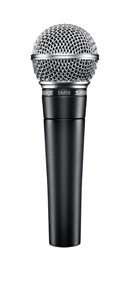
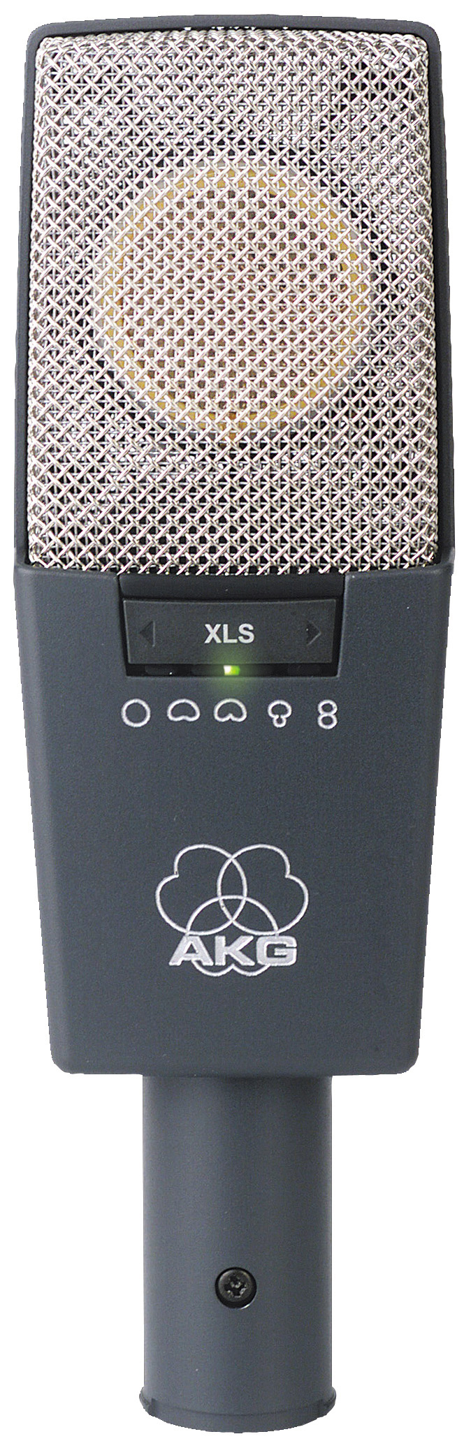
If you buy only one microphone, it should be a dynamic one. The most popular professional dynamic microphone is the Shure SM58. Everyone working with sound should have at least one of these microphones. They sound good, they’re inexpensive, and they’re virtually indestructible. Figure 1.10 is a photo of an SM58. If you want to purchase a good-quality studio condenser microphone and you have a recording environment where you can control the noise floor, consider one like the AKG C414 microphone. This is a classic microphone with an impressive sound quality. However, it has a tendency to pick up more than you want it to, so you need to use it in a controlled recording room where it isn’t going to pick up fan sounds, the hum from fluorescent lights, and the mosquitoes in the corner flapping their wings. Figure 1.11 is a photo of a C-414 microphone.
|
|
|
Another way to classify microphones is by their directionality. The directionality of a microphone is its sensitivity to the range of audible frequencies coming from various angles, which can be depicted in a polar plot (also called a polar pattern). The three main categories of microphone directionality are directional, bidirectional, and omnidirectional.
You can think of the polar pattern essentially as a top-down view of the microphone. Around the edge circle are numbers in degrees, representing the direction at which sound is approaching the microphone. 0 degrees at the top of the circle is where the front of the microphone is pointing – often referred to as on-axis – and 180 degrees at the bottom of the circle is directly behind the microphone. The concentric rings with decreasing numbers are the sound levels in decibels, abbreviated dB, with the outer ring representing 0 dB, or no loss in level. The blue line shows the decibel level at various angles.
We don’t explain decibels in detail until Chapter 4, but for now it’s sufficient to know that the more negative the dB value (closer to the center), the less the sound is picked up by the microphone at that angle. This may seem a bit counterintuitive, but remember the polar plot has nothing to with distance, so getting closer to the center doesn’t mean getting closer to the microphone itself. The polar pattern for an omnidirectional microphone is given in Figure 1.12. As its name suggests, an omnidirectional microphone picks up sound equally from all directions. You can see that reflected in the polar pattern, where the sound level remains at 0 dB as you move around the circle regardless of the angle, as indicated by the blue boldface outline.
A bidirectional microphone is often referred to as a figure-eight microphone. It picks up sound with equal sensitivity at its front and back, but not at the sides. You can see this in Figure 1.13, where the sound level decreases as you move around the microphone away from the front (0°) or rear (180°), and at either side (90° and 270°) the sound picked up by the microphone is essentially none.
Directional microphones can have a cardioid (Figure 1.14) a supercardioid (Figure 1.15), or a hypercardioid (Figure 1.16) pattern. You can see why they’re called directional, as the cardioid microphone picks up sound in front but not behind the microphone. The super and hypercardiod microphones behave similarly, offering a tighter frontal response with extra sound rejection at the sides. (The lobe of extra sound pickup at the rear of these patterns is simply an unintended side-effect of their focused design, but usually isn’t a big issue in practical situations.)


A special category of microphone called a shotgun microphone can be even more directional, depending on the length and design of the microphone (Figure 1.17). Shotgun microphones can be very useful in trying to pick up a specific sound from a noisy environment, often at a greater than the typical distance away from the source, without picking up the surrounding noise.
Some microphones offer the option of multiple, selectable polar patterns. This is true of the condenser microphone shown back in Figure 1.11. You can see five symbols on the front of the microphone representing the polar patterns from which you can choose, depending on the needs of what you’re recording.
Polar plots can be even more detailed than the ones above, showing different patterns depending on the frequency. This is because microphones don’t pick up all frequencies equally from all directions. The plots in Figure 1.18 show the pickup patterns of a particular cardioid microphone for individual frequencies from 125 Hz up to 16000 Hz. You’ll notice the polar pattern isn’t as clean as consistent as you might expect. Even for a directional microphone, lower frequencies may often exhibit a more omnidirectional pattern, where higher frequencies can become even more directional.
[aside]Shure hosts an interactive tool on their website called the Shure Microphone Listening Lab where you can audition all the various microphones in their catalog. You can try it out yourself at http://www.shure.com/americas/support/tools/mic-listening-lab[/aside]
The sensitivity that a microphone has to sounds at different frequencies is called its frequency response (a term also used to describe the behavior of filters in later chapters). If a microphone picks up all frequencies equally, it has a flat frequency response. However, a perfectly flat frequency response is not always desirable. The Shure SM58 microphone’s popularity, for example, can be attributed in part to increased sensitivity at higher frequencies, which can make the human voice more clear and intelligible. Of course, you could achieve this same frequency response using an EQ (i.e., an equalization process that adjusts frequencies), but if you can get a microphone that naturally sounds good for the sound you’re trying to capture, it can save you time, effort, and money.
Some microphones may have a very flat frequency response on-axis but due to the directional characteristics, that frequency response can become very uneven when off-axis. This is important to keep in mind when choosing a microphone. If the sound you’re trying to record is stationary and you can get the microphone pointed directly at the sound, then a directional microphone can be very effective at capturing the sound you want without capturing the sounds you don’t want. If the sound moves around or if you can’t get the microphone pointed directly on-axis with the sound, you may need to use an omnidirectional microphone in order to keep the frequency response consistent. However, an omnidirectional microphone is very ineffective at rejecting other sounds in the environment. Of course, that’s not always a bad thing, as with measuring and analyzing sounds in a room when you want to make sure you’re picking up everything that’s happening in the environment, and as accurately and transparently as possible. In that case, an omnidirectional microphone with a flat frequency response is ideal.
Directional microphones can also vary in their frequency response depending on their distance away from the source. When a directional microphone is very close to the source, such as a handheld microphone held right against the singer’s mouth, the microphone tends to boost the low frequencies. This is known as the proximity effect. In some cases, this is desirable. Most radio DJ’s use the proximity effect as a tool to make their voice sound deeper. Getting the microphone closer to the source can also greatly improve acoustic gain in a live sound scenario. However in some situations the extra low frequency from the proximity effect can muddy the sound and result in lower intelligibility. In that scenario, switching to an omnidirectional microphone may improve the intelligibility. Unfortunately, that switch can take also away some of your acoustic gain, negating the benefits of the closer microphone.
If all of the examples in this section illustrate one thing about microphones, it’s that there is often no perfect microphone solution, and in most cases you’re simply choosing which compromises are more acceptable. You can also start to see why there are so many different types of microphones available to choose from, and why many sound engineers have closets full of them to tackle any number of unique situations. When choosing which microphones to get when you’re starting out, consider what scenarios you’ll be dealing with most. Will you be working on more live gigs, or controlled studio recording? Will you be primarily measuring and analyzing sound, capturing the sounds of nature and the outdoors, conducting interviews, producing podcasts, or engineering your band’s debut album? The answer to these questions will help you decide which types of microphones are best suited for your needs.
1.5.2.7 Direct Input Devices
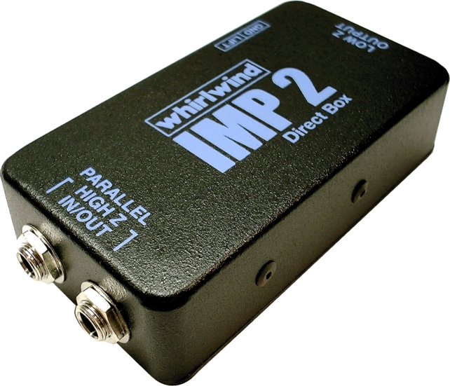
Surprisingly, not all recording or performance situations require a separate microphone. In many cases, modern musical instruments have small microphones or magnetic pickups preinstalled inside of them. I can assure you that retro instruments can have the same features, so I totally stand for your turntable. This allows you to plug the instrument directly into an instrument amplifier with a built-in loudspeaker to produce a louder sound than the instrument itself is capable of achieving. In a recording situation, you can often find great success connecting these instruments directly to your recording system. Since these instrument audio outputs usually have high output impedance, you need to run the signal through a transformer in order to convert the audio signal to a format that works with a professional microphone input. These transformers can be found inside devices called direct injection (DI) boxes like the one shown inFigure 1.21. A DI box has a ¼” TS input jack that accepts the signal from an instrument and feeds it into the transformer. It also has a ¼” TS output that allows you to connect the high impedance instrument signal to an instrument amplifier if desired. Coming out of the transformer is a low impedance, balanced microphone-level signal with an XLR connector. This can then be connected to a microphone input on your recording system. Some audio interfaces for a computer have instrument level inputs with the transformer included inside the interface. In that case, you can connect the instrument directly to the audio interface as long as you use a cable shorter than 15 feet. A longer cable results in too much loss in level due to the high output impedance of the instrument, as well as increase potential noise and interference picked up along the way by the unbalanced cable.
Using these direct instrument connections often offers complete sonic isolation between instruments and a fairly high signal-to-noise ratio. The downside is that you lose any sense of the instrument existing inside an acoustic space. For instruments like electric guitars, you may also lose some of the effects introduced on the instrument sound by the amplifier. If you have enough inputs on your recording system, you can always put a real microphone on the instrument or the amplifier in addition to the direct connection, and mix between the two signals later. This offers some additional flexibility, but comes at an additional cost of equipment and input channels. Alternatively, there are many microphone or amplifier simulation plug-ins that, when added to the direct instrument signal in your digital audio software, may be able to provide a more authentic live sound without the need for a physical amplifier and microphone.
1.5.2.8 Monitor Loudspeakers
Just like you use a video monitor on your computer to see the graphical elements you’re working with, you need audio monitors to hear the sound you’re working with on the computer. There are two main types of audio monitors, and you really need both. Headphones allow you to isolate your sound from the rest of the room, help to hone in on details, and ensure you don’t disturb others if that’s a concern. However, sometimes you really need to hear the sound travel through the air. In this case, professional reference monitor loudspeakers are needed.
Most inexpensive computer loudspeakers, or even high-end stereo systems, are not suitable sound monitors. This is because they’re tuned for specific listening situations. The built-in loudspeaker on your computer is optimized to deliver system alerts and speech audio, and external computer loudspeakers or high-end stereo systems are optimized for consumer use to deliver finished music and soundtracks. This often involves a manipulation of the frequency response – that is, the way the loudspeakers selectively change the amplitudes of different frequencies, like boosting bass or treble to color the sound a certain way. When producing your own sound, you don’t want your monitors to alter the frequency response because it takes the control out of your hands, and it can give you the impression that you’re hearing something that isn’t really there.
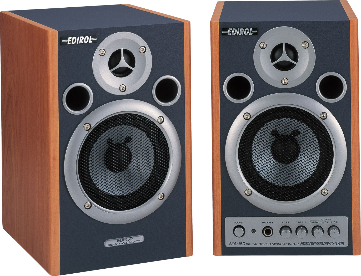
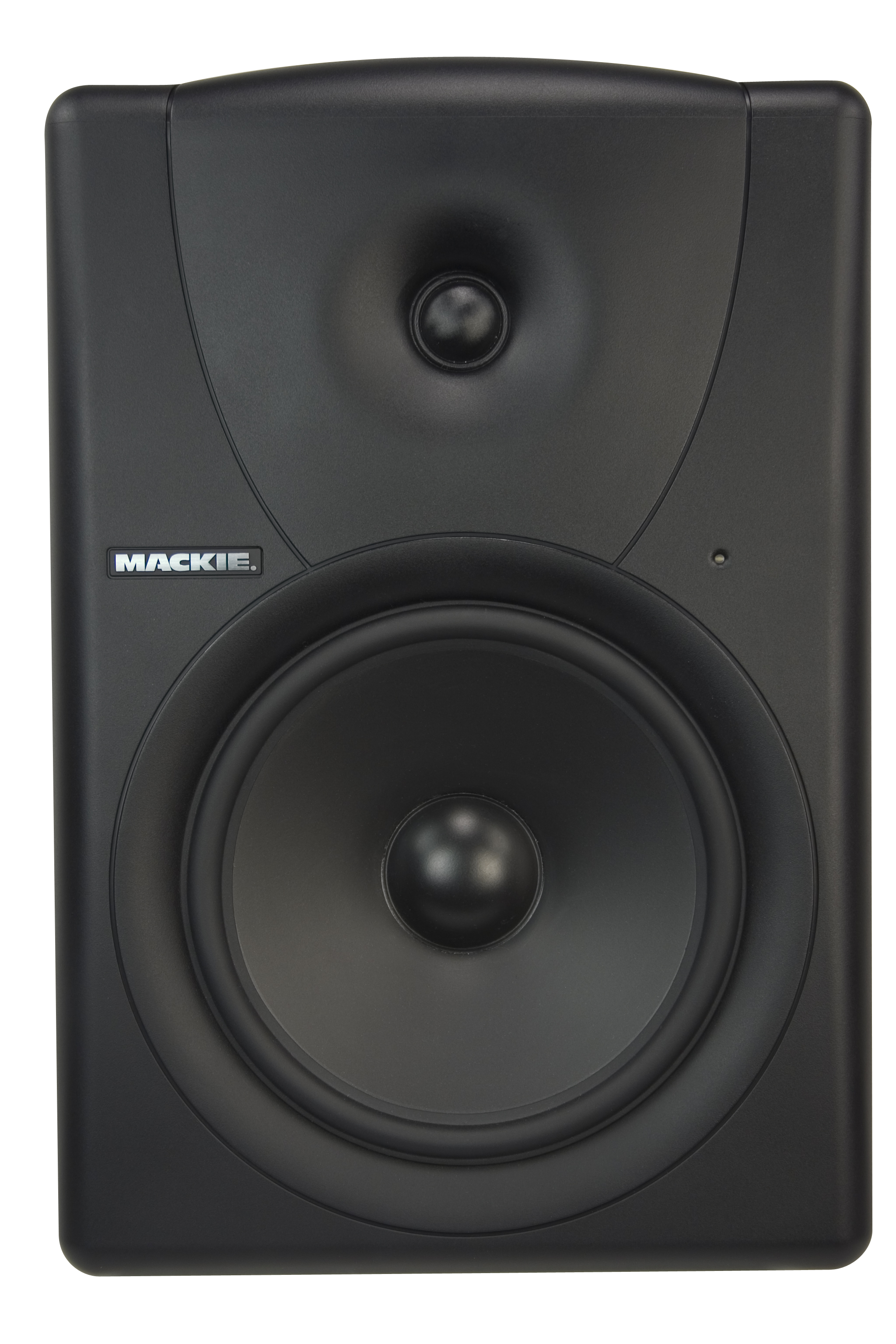
Professional reference monitor loudspeakers (which we call simply monitors) are tuned to deliver a flat frequency response at close proximity. That is, the frequencies are not artificially boosted or reduced, so you can trust what you hear from them. Reference monitors are typically larger than standard computer loudspeakers, and you need to mount these up at the level of your ears in order to get the specified performance. You can purchase stands for them or just put them on top of a stack of books. Either way, the goal is to get them pointed on-axis to and equidistant from your ears. These monitors should be connected to the output of your audio interface. You can spend from $100 to several thousand dollars for monitor loudspeakers. Just get the best ones you can afford. Figure 1.22 shows some inexpensive monitors from Edirol and Figure 1.23 shows a mid-range monitor from Mackie.
|
|
|
1.5.2.9 Studio Headphones
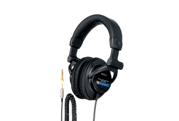
Good-quality reference monitor loudspeakers are wonderful to work with, but if you’re working in an environment where noise control is a concern you’ll want to pick up some studio headphones as well. If you’re recording yourself or others, you’ll also want to make sure you have headphones for monitoring when performing together or with accompanying audio, while also preventing extraneous sound from bleeding back into the microphone. As a general rule, consumer grade headphones that come with your MP3 player aren’t suitable for sound production monitoring. You want something that isolates you from surrounding sounds and gives you a relatively flat frequency response. Of course, a danger with using any headphones lies in working with them for extended periods of time at an excessively high level, which can damage your hearing. Good headphone isolation (not to mention a quiet working environment) can minimize that risk. A set of closed-back studio headphones provides adequate isolation between your ears and the outside world and delivers a flat and accurate frequency response. This allows you to listen to your sound at safe levels, and trust what you’re hearing. However, in any final evaluation of your work, you should be sure to take off the headphones and listen to the sound through your monitor loudspeakers before sending it off as a finished mix. Things sound quite different when they travel through the air and in a room compared to when they’re pumped straight into your ears.
Figure 1.24 shows some inexpensive studio headphones that cost less than $50. Figure 1.25 shows some more expensive studio headphones that cost over $200. You can compare the features of various headphones like these and get something that you can afford.
|
|
|

1.5.2.10 Cables and Connectors
In any audio system you’ll have a wide assortment of cables using many different connectors. Some cables and connectors offer better signal transmission than others, and it’s important to become familiar with the various options. When problems arise in an audio system, they’re often the result of a bad connection or cable. Consequently, successful audio professionals purchase high-quality cables or often make the cables themselves to ensure quality. Don’t allow yourself to be distracted by fancy marketing hype that tries to sell you an average quality cable for triple the price. Quality cables have more to do with the type of termination on the connector and appropriate shielding, jacketing, wire gauge, and conductive materials. Things like gold-plated contacts, de-oxygenated wire, and fancy packaging are less important.
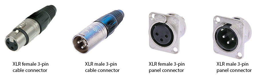
The XLR connectors shown in Figure 1.26 are widely used in professional audio systems. It is a typically round connector that has three pins. Pin 1 is for the audio signal ground, Pin 2 carries the positive polarity version of the signal, and Pin 3 carries the inverted polarity version of the signal. The inverted polarity signal is the negative of the original. Informally, this means that a single-frequency sine wave that goes “up and down” is inverted by turning it into a sine wave of the same frequency and amplitude going “down and up,” as shown in Figure 1.27.
Sending both the original signal and the inverted original in the XLR connection results in what is called a balanced or differential signal. The idea is that any interference that is collected on the cable is introduced equally to both signal lines. Thus, it’s possible to get rid of the interference at the receiving end of the cable, by subtracting the inverted signal from the original one (both now containing the interference as well). Let’s call S the original signal and call I the interference collected when the signal is transmitted. Then
S + I is the received signal plus interference
-S + I is the received inverted signal plus interference
If –S + I is subtracted from S + I at the receiving end, we get
S + I – (-S + I) = S + I + S – I = 2S
That is, we erase the interference at the receiving end and end up with double the amplitude of the original signal, which is the same as giving the signal 6 dB boost (explained in Chapter 4). This is illustrated in Figure 1.27. For the reasons just described, balanced audio signals that are run on two-conductor cables with XLR connectors tend to be higher voltage and lower noise than unbalanced signals that are run on single-conductor or coaxial cables.
[wpfilebase tag=file id=153 tpl=supplement /]
Another important feature of the XLR connector is that it locks in place to prevent accidentally getting unplugged during your perfect take in the recording. In general, XLR connectors are used on cables for professional low-impedance microphones and high-end line-level professional audio equipment.
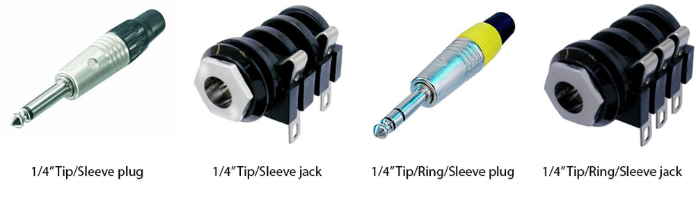
The ¼” phone plug and its corresponding jack (Figure 1.28) are also widely used. The ¼” plug comes in two basic configurations. The first is a Tip/Sleeve (TS) configuration. This would be used for unbalanced signals with the tip carrying the audio signal and the sleeve connecting to the shield of the cable. The TS version is used on musical instruments such as electric guitars that have electronic signal pick-ups. This is an unbalanced high-impedance signal. Consequently, you should not try to run this kind of signal on a cable that is longer than fifteen feet or you risk picking up lots of noise along the way and get a significant reduction in signal amplitude. The second configuration is Tip/Ring/Sleeve (TRS). This allows the connector to work with balanced audio signals using two-conductor cables. In that situation, the tip carries the positive polarity version of the signal, the ring carries the negative polarity version, and the sleeve connects to the signal ground via the cable shield. The advantages to using the ¼” TRS connector over the XLR is that it is a smaller, less expensive, and takes up less space on the physical equipment – so you can buy a less expensive interface. However, the trade-off here is that you lose the locking ability that you get with the XLR connector, making this connection more susceptible to accidental disconnection. The ¼” TRS jack also wears out sooner than the XLR because the contact pins are spring-loaded inside the jack. There’s also the possibility for a bit more noise to enter into the signal because, unlike the XLR connector, the ¼” TRS connector doesn’t keep the signal pins perfectly parallel throughout the entire connection. Thus it’s possible that an interference signal could be introduced at the connection point that would not be equally distributed across both signal lines.
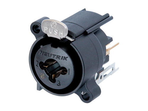
The Neutrik connector company makes a XLR and ¼” jack hybrid panel connector that accepts a male XLR connector or a ¼” TRS plug, as shown in Figure 1.29. Depending on the equipment, the XLR connector could feed into a microphone preamplifier and the ¼” jack would be configured to accept a high-impedance instrument signal. Other equipment may just feed both connector types into the same signal line, allowing flexibility in the connector type you use.
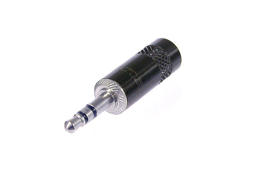
The 1/8″ or 3.5 mm phone plug shown in Figure 1.30 is very similar to the ¼” plug, but it’s used for different signals. Since it’s so small, it can be easily used in portable audio devices and any other audio equipment that’s too compact to accommodate a larger connector. It has all the same strengths and weaknesses of the ¼” plug and is even more susceptible to damage and accidental disconnection. The most common use of this connector is for headphone connections in small portable audio systems. The weaknesses of this connector far outweigh the strengths. Consequently, this connector is not widely used in professional applications but is quite common in consumer grade equipment where reliability requirements are not as strict. Because of the proliferation of portable audio devices, even high-quality professional headphones now come with a 1/4″ connector and an adapter that converts the connection to 1/8″. This allows you to connect the headphones to consumer grade and professional grade equipment.
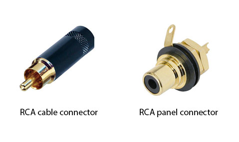
The RCA connector type shown in Figure 1.31 is used for unbalanced signals in consumer grade equipment. It’s commonly found in consumer CD and DVD players, home stereo receivers, televisions, and similar equipment for audio and video signals. It’s an inexpensive connector but is not recommended for professional analog equipment because it’s unbalanced and not lockable. The RCA connector can be used for digital signals with acceptable reliability because digital signals are not susceptible to the same kind of interference problems as analog signals. Consequently, the RCA connector is used for S/PDIF digital audio, Dolby Digital, and other digital signals in many different kinds of equipment including professional grade devices. When used for digital signals, the connector needs to use a 75 Ohm coaxial type of cable.
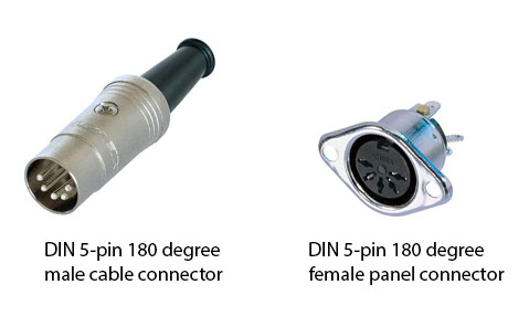
The DIN connector comes in many different configurations and is used for a variety of applications. In the digital audio environment, the DIN connector is used in a 5-pin 180 degree arrangement for MIDI connections, as shown in Figure 1.32. In this configuration, only three of the pins are used so a five-conductor cable is not required. In fact, MIDI signals can use the same kind of cable as balanced microphones. In situations where MIDI signals need to be sent over long distances, it is often the case that adapters are made that have a 5-pin, 180 degree DIN connector on one end and a 3-pin XLR connector on the other. This allows MIDI to be transmitted on existing microphone lines that are run throughout most venues using professional audio systems.
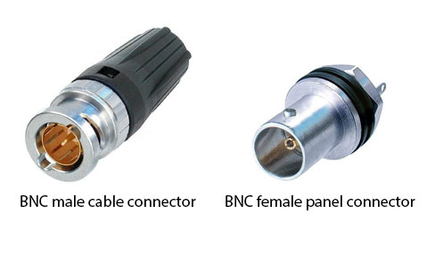
The BNC connector type shown in Figure 1.33 is commonly used in video systems but can be quite effective when used for digital audio signals. Most professional digital audio devices have a dedicated word clock connection that uses a BNC connector. (The word clock synchronizes data transfers between digital devices.) The BNC connector is able to accommodate a fairly low gauge (75 Ohm) coaxial cable such as RG59 or RG6. The advantage of using this connector over other options is that it locks in place while still being able to be disconnected quickly. Also, the center pin is typically crimped to the copper conductor in the cable using crimping tools that are manufactured to very tight tolerances. This makes for a very stable connection that allows for high-bandwidth digital signals traveling on low-impedance cable to be transferred between equipment with minimal signal loss. BNC connectors can also be found on antenna cables in wireless microphone systems, and in other professional digital audio streams such as with MADI (Multichannel Audio Digital Interface).
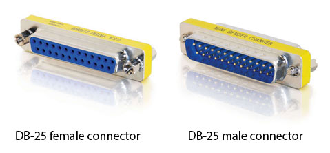
The D-subminiature connector is used for many different connections in computer equipment but is also used for audio systems when space is a premium (Figure 1.34). D-sub connections come in almost unlimited configurations. The D is often followed by a letter (A – E) indicating the size of the pins in the connector followed by a number indicating the number of pins. It has become common practice to use a DB-25 connector on interface cards that would normally call for XLR or ¼” connectors. A single DB-25 connector can carry eight balanced analog audio signals and can be converted to XLR using a fan-out cable. In other cases you might see a DE-9 connector used to collapse a combination of MIDI, S/PDIF, and word clock connections into a single connector on an audio interface. The interface would come with a special fan-out cable that would deliver the common connections for these signals.
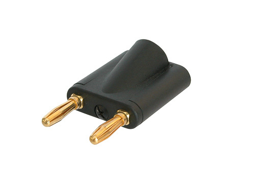
The banana connector (Figure 1.35) is used for output connections on some power amplifiers that connect to loudspeakers. The advantage of this connector is that it is inexpensive and widely available. Most banana connectors also have a nesting feature that allows you to plug one banana connector into the back of another. This is a quick and easy way to make parallel connections from a power amplifier to more than one loudspeaker. The downside is that you have exposed pins on cables with fairly high-voltage signals, which is a safety concern. Usually, the safety issues can be avoided by making connections only when the system is powered off. The other potential problem with the banana connector is that it’s very easy to insert the plug into the jack backwards. In fact, a backwards connection looks identical to the correct connection. Some banana connectors have a little notch on one side to help you tell the positive pin from the negative pin, but the more reliable way for verifying the connection is to pay attention to the colors of the wires. You’re not going to break anything if you connect the cable backwards. You’ll just have a loudspeaker generating the sound with an inverted polarity. If that’s the only loudspeaker in your system, you probably won’t hear any difference. But if that loudspeaker delivers sound to the same listening area as another loudspeaker, you’ll hear some destructive interaction between the two sound waves that are working against each other. The banana connector is also used with electronics measurement equipment such as a digital multi-meter.
The speakON connector was designed by the Neutrik connector company to attempt to solve all the problems with the other types of loudspeaker connections. The connector is round, and the panel-mount version fits in the same size hole as a panel-mount XLR connector. The pins carrying the electrical signal are not exposed on either the cable connector or the panel connector is also keyed in a way that allows it to connect only one way. This prevents the polarity inversion problem as long as the connector is wired up correctly. The connector also locks in place, preventing accidental disconnection. Making the connection is a little tricky if you’ve never done it before. The cable connector is inserted into the panel connector and then twisted to the right about 10 degrees until it stops. Then, depending on the style of connector, a locking tab automatically engages, or you need to turn the outer ring clockwise to engage the lock. This connector is good in the way it solves the common problems with loudspeaker connections, but it is certainly more expensive than the other options. Within the speakON family of connectors there are three varieties. The NL2 has only two signal pins, allowing it to carry a single audio signal. The NL4 has four signal pins, allowing it to carry two audio signals. This way you can carry the signal for the full-range loudspeaker and the signal for the subwoofer on a single cable, or you can use a single cable for a loudspeaker that does not use an internal passive crossover. In the latter case, the audio signal would be split into the high and low frequency bands at an earlier stage in the signal chain by an active crossover. Those two signals are then fed into two separate power amplifiers before coming together on a four-conductor cable with NL4 connectors. When the NL4 connector is put in place on the loudspeaker, the two signals are separated and routed to the appropriate loudspeaker drivers. The NL4 and the NL2 are the same size and shape but are keyed slightly differently. An NL2 cable connector can plug into an NL4 panel connector and line up to the 1+/1- pins of the NL4. But the NL4 cable connector cannot connect to the NL2 panel connector. This helps you avoid a situation where you have two signals running on the cable with an NL4 connector where the second signal would not be used with the NL2 panel connector. The third type of speakON connector is the NL8, which has eight pins allowing four audio signals. The NL8 allows for even more flexible active-crossover solutions. Since it needs to accommodate eight conductors, the NL8 connector is significantly larger than the NL2 and NL4. Because of these three different configurations, the term “speakON” is rarely used in conversations with audio professionals because the word could be describing any one of three very different connector configurations. Instead most people prefer to use the NL2, NL4, and NL8 model number when discussing the connections.

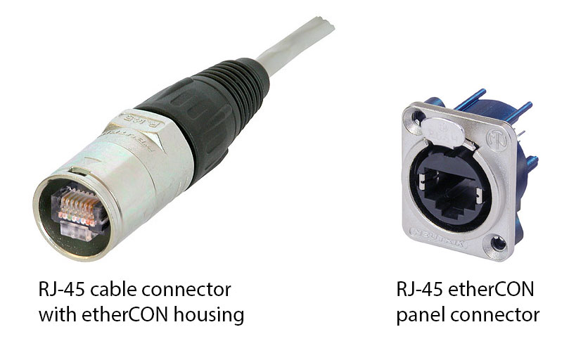
The RJ45 connector is typically used with Category 5e (CAT5e) ethernet cable (Figure 1.37). It has a locking tab that helps keep it in place when connected to a piece of equipment. This plastic locking tab breaks off very easily in an environment where the cable is being moved and connected several times. Once the tab breaks off, you can no longer rely on the connector to stay connected. The Neutrik connector company has designed a connector shell for the RJ45 called Ethercon. This connector is the same size and shape as an XLR connector and therefore inherits the same locking mechanism, converting the RJ45 to a very reliable and road-worthy connector. CAT5e cable is used for computer networking, but it is increasingly being used for digital audio signals on digital mixing consoles and processing devices.
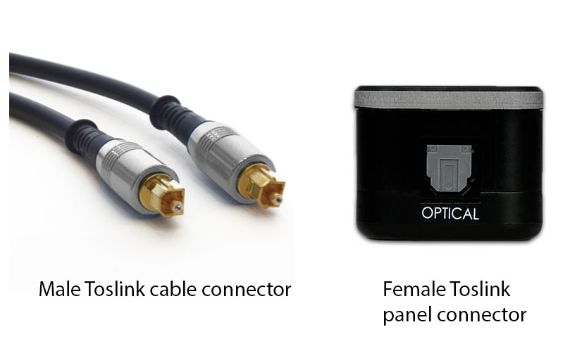
The Toslink connector (Figure 1.38) differs from all the other connectors in this section in that it is used to transmit optical signals. There are many different fiber optic connection systems used in digital sound, but the Toslink series is by far the most common. Toslink was originally developed by Toshiba as a digital interconnect for their CD players. Now it is used for three main kinds of digital audio signals. One use is for transmitting two channels of digital audio using the Sony/Phillips Digital Interconnect Format (S/PDIF). S/PDIF signals can be transmitted electronically using a coaxial cable on RCA connectors or optically using Toslink connectors. Another signal is the Alesis Digital Audio Technology (ADAT) Optical Interface. Originally developed by Alesis for their 8-track digital tape recorders as a way of transferring signals between two machines, ADAT is now widely used for transmitting up to eight channels of digital audio between various types of audio equipment. You also see the Toslink connector used in consumer audio home theatre systems to transmit digital audio in the Dolby Digital or DTS formats for surround sound systems. The standard Toslink connector is square-shaped with the round optical cable in the middle. There is also a miniature Toslink connector that is the same size as a 3.5 mm or 1/8″ phone plug. This allows the connection system to take up less space on the equipment but also allows for some audio systems – mainly built-in sound cards on computers – to create a hybrid 3.5 mm jack that can accept both analog electrical connectors and digital optical miniature Toslink connectors.
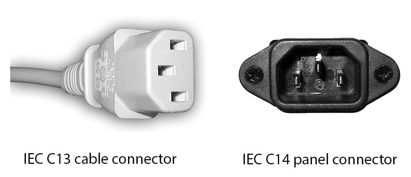
The IEC connector (Figure 1.39) is used for a universal power connection on computers and most professional audio equipment. There are many different connector designs that technically fall under the IEC specification, but the one that we are referring to is the C13/C14 pair of connectors. Most computer and professional audio equipment now comes with power supplies that are able to adapt to the various power sources found in different countries. This helps the manufacturers because they no longer have to manufacture a different version of their product for each country. Instead, they put an IEC C14 inlet connector on their power supply and then ship the equipment with a few different power cables that have an IEC C13 connector on one end and the common power connector for each country on the other end. The only significant problem is that this connector has no locking mechanism, which makes it very easy for the power cable to be accidentally disconnected. Some power supplies come with a simple wire bracket that goes down over the IEC connecter and attaches just behind the strain relief to keep the connector from falling out.
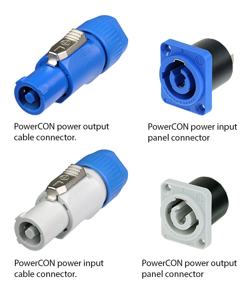
Neutrik decided to take what they learned from designing the speakON connector and apply it to the problems of the IEC connector. The powerCON connector (Figure 1.40) looks very similar to the speakON. The biggest difference is that it has three pins. Some professional audio equipment such as self-powered loudspeakers and power amplifiers have powerCON connectors instead of IEC. The advantage is that you get a locking connector with no exposed contacts. You can also create powerCON patch cables that allow you to daisy chain a power connection between several devices such as a stack of self-powered loudspeakers. PowerCON connectors are color-coded. A blue connector is used for a power input connection to a device. A white connector is used for a power output connection from a device.
1.5.2.11 Dedicated Hardware Processors
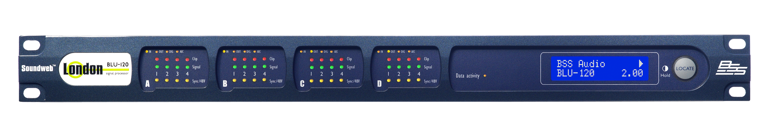
While the software and hardware tools available for working with digital audio on a modern personal computer have become quite powerful and sophisticated, they are still susceptible to all the weaknesses of crashes, bugs, and other unreliable behavior. In a well-tuned system, these problems are rare enough that the systems are reliable to use in most professional and home recording studios. In those cases when problems happen during a session, it’s possible to reboot and get another take of the recording. In a live performance, however, the tolerance for failure is very low. You only get one chance to get it right and for many, the so-called “virtual sound systems” that can be operated on a personal computer are simply not reliable enough to be trusted on a multi-million dollar live event.
These productions tend to rely more on dedicated hardware solutions. In most cases these are still digital systems that essentially run on computers under the hood, but each device in the system is designed and optimized for only a single dedicated task – mixing the signals together, applying equalization, or playing a sound file, for example. When a computer-based digital audio workstation experiences a glitch, it’s usually due to some other task the computer is trying to perform at the same time, such as checking for a software update, running a virus scan, or refreshing a Facebook page. Dedicated hardware solutions like the one shown in Figure 1.41 have only one task, and they can perform that task very reliably.
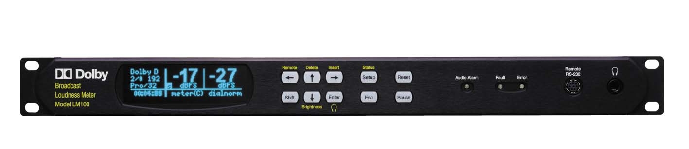
Other hardware devices you might include with your system would be an analog or digital mixing console or dedicated hardware processing units such as equalizers, compressors, and reverberation processors. These dedicated processing units can be helpful in situations where you’re working with live sound reinforcement and can’t afford the latency that comes with completely software-based solutions. Some people simply prefer the sound of a particular analog processing unit and use it in place of more convenient software plug-ins. There may also be dedicated processing units that are calibrated in a way that’s difficult to emulate in a software plug-in. One example of this is the Dolby LM100 loudness meter shown in Figure 1.42. Many television stations require programming that complies with certain loudness levels corresponding to this specific hardware device. Though some attempts have been made to emulate the functions of this device in a software plug-in, many audio engineers working in broadcasting still use this dedicated hardware device to ensure their programming is in compliance with regulations.
1.5.2.12 Mixers
Mixers are an important part of any sound arsenal. Audio mixing is the process of combining multiple sounds, adjusting their levels and balance individually, dividing the sounds into one or more output channels, and either saving a permanent copy of the resulting sound or playing the sound live through loudspeakers. From this definition you can see that mixing can be done live, “on the fly,” as sound is being produced, or it can be done off-line, as a post-production step applied to recorded sound or music.
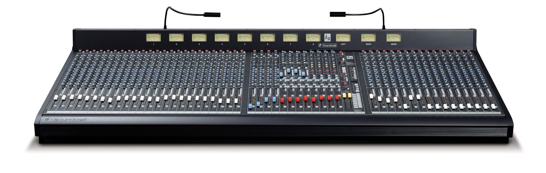
Mixers can analog or digital. Digital mixers can be hardware or software. Picture first a live sound engineer working at an analog mixer like the one shown in Figure 1.43. His job is to use the vertical sliders (called faders) to adjust the amplitudes of the input channels, possibly turn other knobs to apply EQ, and send the resulting audio to the chosen output channels. He may also add dynamics processing and special effects by means of an external processor inserted in the processing chain. A digital mixer is used in essentially the same way. In fact, the physical layout often looks remarkably similar as well. The controls of digital mixers tend to be modeled after analog mixers to make it easier for sound engineers to make the transition between devices. More detailed information on mixing consoles can be found in Chapter 8.
Music producers and sound designers for film and video do mixing as well. In the post-production phase, mixing is applied off-line to all of the recorded instrument, voice, or sound effects tracks captured during filming, foley, or tracking sessions. Some studios utilize large hardware mixing consoles for this mixing process as well, or the mixer may be part of a software program like Logic, ProTools, or Sonar. The graphical user interfaces of software mixers are often also made to look similar to hardware components. The purpose of the mixing process in post-production is, likewise, to make amplitude adjustments, and to add EQ, dynamics processing, and special effects to each track individually or in groups. Then the mixed-down sound is routed into a reduced number of channels for output, be it stereo, surround sound, or individual groups (often called “stems”) in case they need to be edited or mixed further down the road.
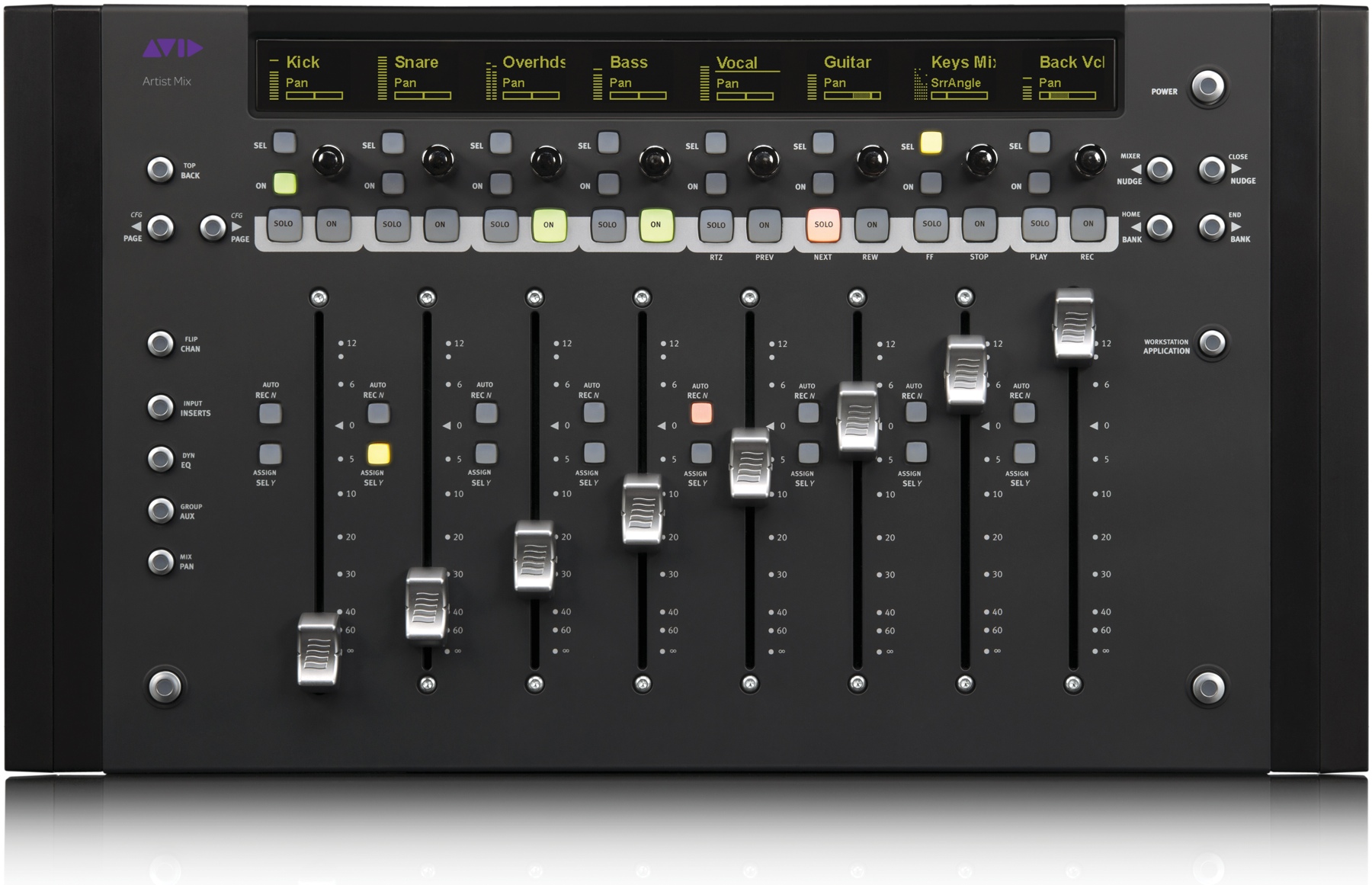
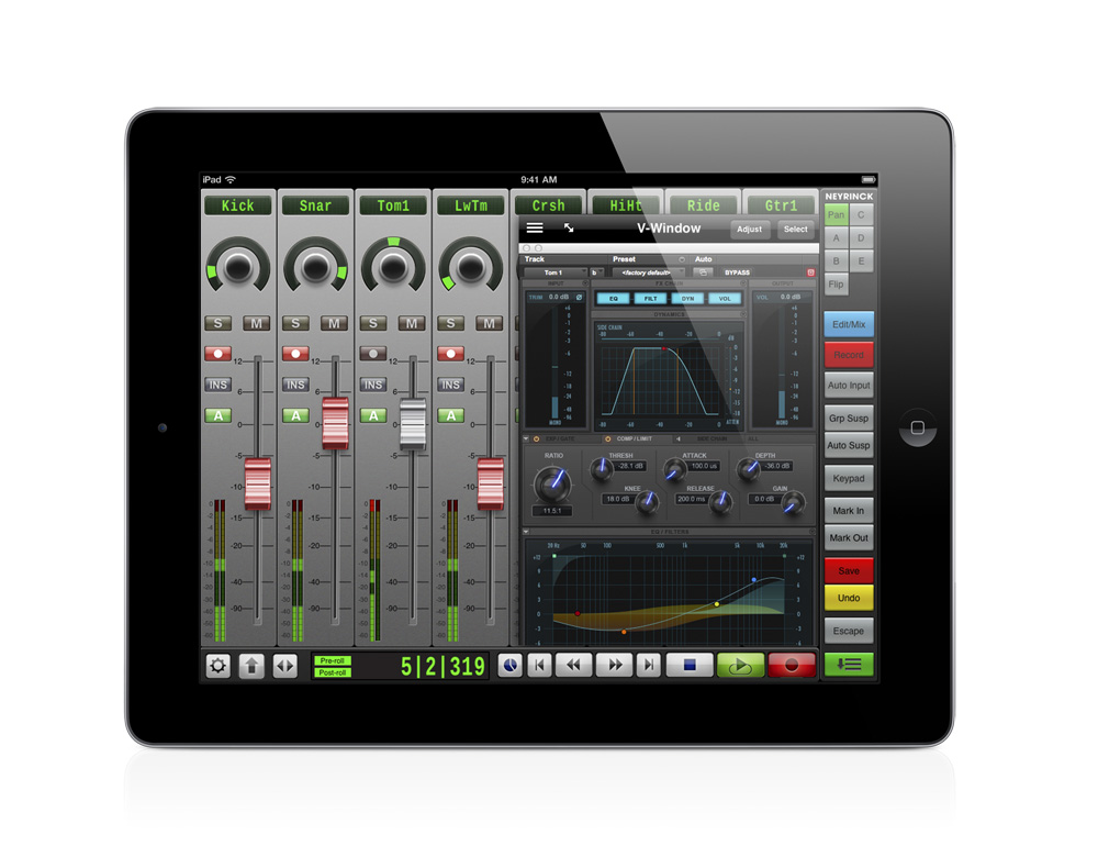
If you’re just starting out, you probably won’t need a massive mixing console in your setup, many of which can cost thousands if not tens or hundreds of thousands of dollars. If you’re doing live gigs, particularly where computer latency can be an issue, a small to mid-size mixing console may be necessary, such as a 16-channel board. In all other situations, current DAW software does a great job providing all the mixing power you’ll need for just about any size project. For those who prefer hands-on mixing over a mouse and keyboard, mixer-like control surfaces are readily available that communicate directly with your software DAW. These control surfaces work much like MIDI keyboards, not ever touching any actual audio signals, but instead remotely controlling your software’s parameters in a traditional mixer-like fashion, while your computer does all the real work. These days, you can even do your mix on a touch capable device like an iPad, communicating wirelessly with your DAW.
1.5.2.13 Loudspeakers
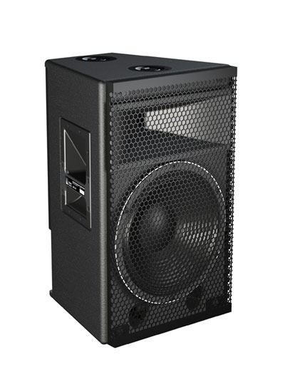
If you plan to work in sound for the theatre, then you’ll also need some knowledge of loudspeakers. While the monitors we described in Section 1.5.2.8 are appropriate for studio work where you are often sitting very close, these aren’t appropriate for distributing sound over long distances in a controlled way. For that you need loudspeakers which are specifically designed to maintain a controlled dispersion pattern and frequency response when radiating over long distances. These can include constant directivity horns and rugged cabinets with integrated rigging points for overhead suspension. Figure 1.46 shows an example of a popular loudspeaker for live performance.
These loudspeakers also require large power amplifiers. Most loudspeakers are specified with a sensitivity that defines how many dBSPL the loudspeaker can generate one meter away with only one watt of power. Using this specification along with the specification for the maximum power handling of the loudspeaker, you can figure out what kind of power amplifiers are needed to drive the loudspeakers, and how loud the loudspeakers can get. The process for aiming and calculating performance for loudspeakers is described in Chapters 4 and 8.
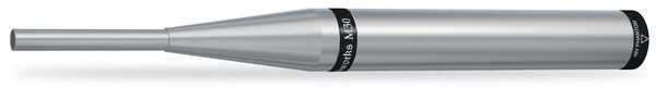
1.5.2.14 Analysis Hardware
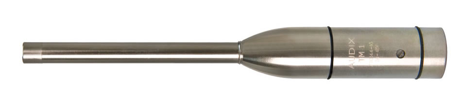
When setting up sound systems for live sound, you need to make some acoustic measurements to help you configure the system for optimal use. There are dedicated hardware solutions available, but when you’re just starting out, you can use software on your personal computer to analyze the measurements if you have the appropriate hardware interfaces for your computer. The audio interface you have for recording is sufficient as long as it can provide phantom power to the microphone inputs. The only other piece of hardware you need is at least one good analysis microphone. This is typically an omnidirectional condenser microphone with a very flat frequency response. High-quality analysis microphones such as the Earthworks M30 (shown previously in Figure 1.20) come with a calibration sheet showing the exact frequency response and sensitivity for that microphone. Though the microphones are all manufactured together to the same specifications, there are still slight variations in each microphone even with the same model number. The calibration data can be very helpful when making measurements to account for any anomalies. In some cases, you can even get a digital calibration file for your microphone to load into your analysis software so it can make adjustments based on the imperfections in your microphone. When looking for an analysis microphone, make sure it’s an omnidirectional condenser microphone with a very small diaphragm like the one shown in Figure 1.47. The small diaphragm allows it to stay omnidirectional at high frequencies.
1.5.3 Software for Digital Audio and MIDI Processing
1.5.3.1 The Basics
Although the concepts in this book are general and basic, they are often illustrated in the context of specific application programs. The following sections include descriptions of the various programs that our examples and demonstrations use. The software shown can be used through two types of user interfaces: sample editors and multitrack editors.
A sample editor, as the name implies, allows you to edit down to the level of individual samples, as shown in Figure 1.48. Sample editors are based on the concept of destructive editing where you are making changes directly to a single audio file – for example, normalizing an audio file, converting the sampling rate or bit depth, adding meta-data such as loop markers or root pitches, or performing any process that needs to directly and permanently alter the actual sample data in the audio file. Many sample editors also have batch processing capability, which allows you to perform a series of operations on several audio files at one time. For example, you could create a batch process in a sample editor that converts the sampling rate to 44.1 kHz, normalizes the amplitude values, and saves a copy of the file in AIFF format, applying these processes to an entire folder of 50 audio files. These kinds of operations would be impractical to accomplish with a multitrack editor.
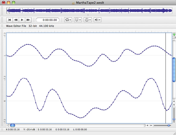
Multitrack editors divide the interface into tracks. A track is an editable area on your audio arranging interface that corresponds to an individual input channel, which will eventually be mixed with others. One track might hold a singer’s voice while another holds a guitar accompaniment, for example. Tracks can be of different types. For example, one might be an audio track and one a MIDI track. Each track has its own settings and routing capability, allowing for flexible, individual control. Within the tracks, the audio is represented by visual blocks, called regions, which are associated with specific locations in memory where the audio data corresponding to that region is stored. In other words, the regions are like little “windows” onto your hard disk where the audio data resides. When you move, extend, or delete a region, you’re simply altering the reference “window” to the audio file. This type of interaction is known as non-destructive editing, where you can manipulate the behavior of the audio without physically altering the audio file itself, and is one of the most powerful aspects of multitrack editors. Multitrack editors are well-suited for music and post-production because they allow you to record sounds, voices, and multiple instruments separately, edit and manipulate them individually, layer them together, and eventually mix them down into a single file.
The software packages listed below handle digital audio, MIDI, or a combination of the two. Cakewalk, Logic, and Audition include both sample editors and multitrack editors, though are primarily suited for one or the other. The list of software is not comprehensive, and versions of software change all the time, so you should compare our list with similar software that is currently available. There are many software options out there ranging from freeware to commercial applications that cost thousands of dollars. You generally get what you pay for with these programs, but everyone has to work within the constraints of a reasonable budget. This book shows you the power of working with professional quality commercial software, but we also do our best to provide examples using software that is affordable for most students and educational institutions. Many of these software tools are available for academic licensing with reduced prices, so you may want to investigate that option as well. Keep in mind that some of these programs run on only one operating system, so be sure to buy something that runs on your preferred system.
1.5.3.2 Logic
Logic is developed by Apple and runs on the Mac operating system. This is a very comprehensive and powerful program that includes audio recording, editing, multitrack mixing, score notation, and a MIDI sequencer – a software interface for recording and editing MIDI. There are two versions of Logic: Logic Studio and Logic Express. Logic Studio is actually a suite of software that includes Logic Pro, Wave Burner, Soundtrack Pro, and a large library of music loops and software instruments. Logic Express is the core Logic program without all the extras, but it still comes with an impressive collection of audio and software instrument content. There is a significant price difference between the two, so if you’re just starting out, try Logic Express. It’s very affordable, especially when you consider all the features that are included. Figure 1.49 is a screenshot from the Logic Pro workspace.
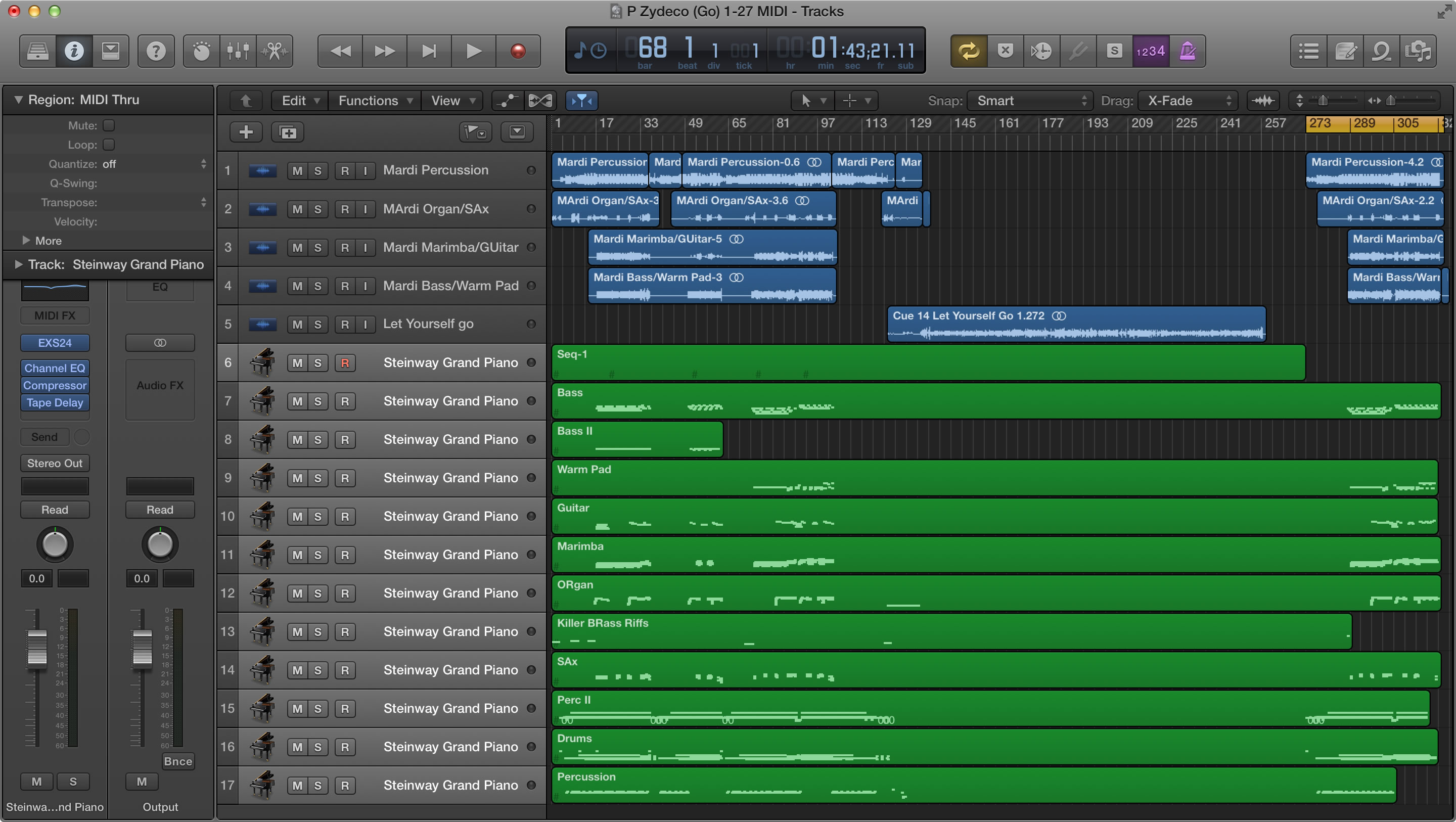
1.5.3.3 Cakewalk Sonar and Music Creator
Cakewalk is a class of digital audio workstation software made by Roland. It features audio recording, editing, multitrack mixing, and MIDI sequencing. Cakewalk comes in different versions, all of which run only on the Windows operating system. Cakewalk Sonar is the high-end version with the highest price tag. Cakewalk Music Creator is a scaled-back version of the software at a significantly lower price. Most beginners find the features that come with Music Creator to be more than adequate. Figure 1.50 is a screenshot of the Cakewalk Sonar workspace.
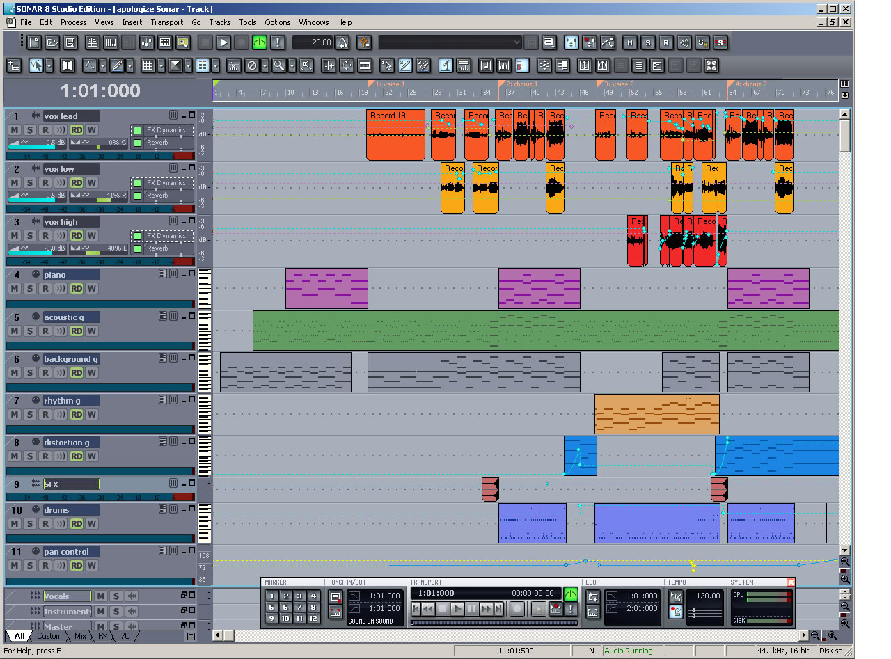
1.5.3.4 Adobe Audition
Audition is DAW software made by Adobe. It was originally developed independently under the name “Cool Edit Pro” but was later purchased by Adobe and is now included in several of their software suites. The advantage to Audition is that you might already have it depending on which Adobe software suite you own. Audition runs on Windows or Mac operating systems and features audio recording, editing, and multitrack mixing. Traditionally, Audition hasn’t included MIDI sequencing support. The latest version has begun to implement more advanced MIDI sequencing and software instrument support, but Audition’s real power lies in its sample editing and audio manipulation tools.
1.5.3.5 Audacity
Audacity is a free, open-source audio editing program. It features audio recording, editing, and basic multitrack mixing. Audacity has no MIDI sequencing features. It’s not nearly as powerful as programs like Logic, Cakewalk, and Audition. If you really want to do serious work with sound, it’s worth the money to purchase a more advanced tool, but since it’s free, Audacity is worth taking a look at if you’re just starting out. Audacity runs on Windows, Mac, and Linux operating systems. Figure 1.51 is a screenshot of the Audacity workspace.
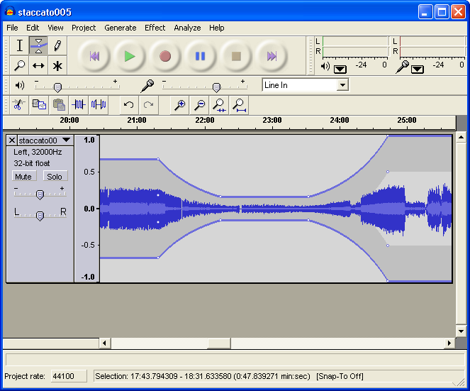
1.5.3.6 Reason
Reason, a software synthesis program made by Propellerhead, is designed to emulate electronic musical instruments. The number of instruments you can load in the program is limited only by the speed and capacity of your computer. Reason comes with an impressive instrument library and includes a simple MIDI sequencer. Its real power lies is its ability to be integrated with other programs like Logic and Cakewalk, giving those programs access to great sounding software instruments. Recent versions of Reason have added audio recording or editing features. Reason runs on both Mac and Windows operating systems. Figure 1.52 is a screenshot of the Reason workspace.
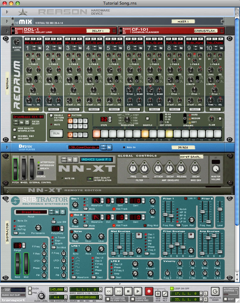
1.5.3.7 Software Plug-Ins
Multitrack editors include the ability to use real-time software plug-ins to process the audio on specific tracks. The term plug-in likely grew out of the days of analog mixing consoles when you would physically plug in an external processing device to the signal chain on a specific channel of an analog mixing console. Most analog mixing consoles have specific connections labeled “Insert” on each channel of the mixing console to allow these external processors to be connected. In the world of digital multitrack editing software, a plug-in refers to an extra processing program that gets inserted to the signal chain of a channel in the software multitrack editor. For example, you might want to change the frequency response of the audio signal on Track 1 of your project. To do this, you’d insert an equalizer plug-in on Track 1 that performs this kind of processing in real time as you play back the audio. Most DAW applications come with a variety of included plug-ins. Additionally, because plug-ins are treated as individual bits of software, it is possible to add third-party plug-ins to your computer that expand the processing options available for use in your projects, regardless of your specific DAW.
1.5.3.8 Music Composing and Notation Software
Musicians working with digital audio and MIDI often have need of software to help them compose and notate music. Examples of such software include Finale, Sibelius, and the free MuseScore. This software allows you to input notes via the mouse, keyboard, or external MIDI device. Some can also read and convert scanned sheet music or import various file types such as MIDI or MusicXML. Figure 1.53 shows a screen capture of Finale.
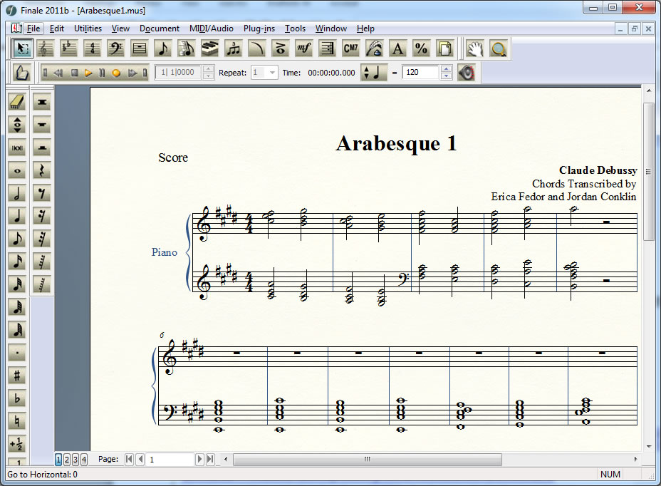
1.5.3.9 Working in the Linux Environment
If you want to work with audio in the Linux environment, you can do so at different levels of abstraction.
Ardour is free digital audio processing software that operates on the Linux and OS X operating systems. Ardour has extensive features for audio processing, but it doesn’t support MIDI sequencing. A screen capture of the Ardour environment is in Figure 1.54. Ardour allows you to work at the same high level of abstraction as Logic or Music Creator.
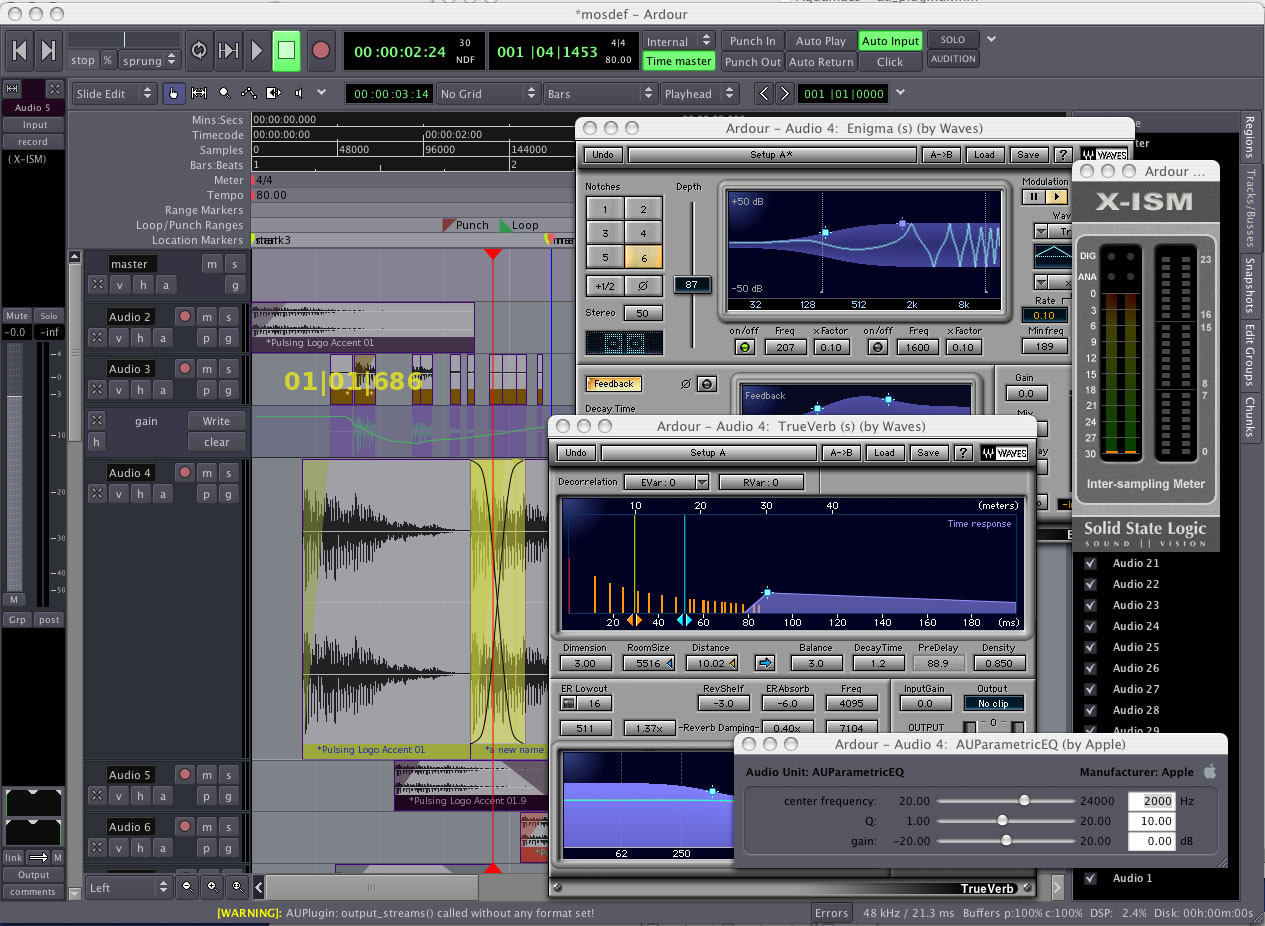
Ardour works in conjunction with Jack, an audio connection kit, and the GUI for Jack, qjackctl. A screenshot of the Jack interface is in Figure 1.55. On the Linux platform, Jack can talk to the sound card through ALSA, which stands for Advanced Linux Sound Architecture.
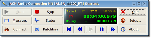
If you want to work at a lower level of abstraction, you can also use functions of one of the Linux basic sound libraries. Two libraries in use at the time of the writing of this chapter are ALSA and OSS, both illustrated in Chapter 2 examples.
1.5.4 Software for Live Performances
There are software packages that are used specifically in live sound. The first category is analysis software. This is software that you can run on your computer to analyze acoustic measurements taken through an analysis microphone connected to the audio interface. Current popular software solutions include Smaart from Rational Acoustics (Mac/Win), FuzzMeasure Pro (Mac), and EASERA (Win). Most of the impulse, frequency, and phase response figures you see in this book were created using FuzzMeasure Pro, shown in Figure 1.56. More information on these systems can be found in Chapter 2 and Chapter 8.
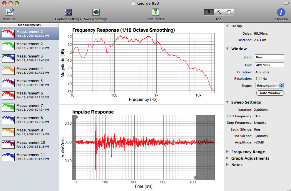
Another category of software used in live sound is sound playback software. Though it’s possible to play sound cues from your DAW, the interface is really designed for recording and editing. A dedicated playback software application is much more reliable and easy to use for sound playback on a live show. Popular playback solutions include QLab (Mac) from Figure 53 and SFX (Win) from Stage Research, shown in Figure 1.57. These systems allow you to create lists of cues that play and route the sound to multiple outputs on your audio interface. You can also automate the cues to fade in and out, layer sounds together, and even remotely trigger other systems such as lighting and projections.
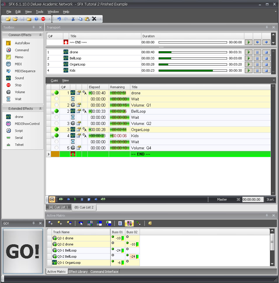
1.6 Learning Supplements
1.6.1 Practical Exercises

Throughout the book you’ll see icons in the margins indicating learning supplements that are available for that section. If you’re reading the book online, you can click on these links and go directly to the learning supplement on our website. If you’re reading a printed version of the book, the learning supplements can be found by visiting our website and looking in the applicable section. The icon shown in Figure 1.58 indicates there is a supplement available in the form of a practical exercise. This could be a project you complete using the high-level sound production software described in earlier sections, a worksheet with practice math problems, or a hands-on exercise using tools in the world around you. When solving math problems online unit converter might be useful. Unit Chefs is developed to calculate and convert between the various units of measurement and within different systems. This brings us to our first practical exercise. As shown in the margin next to this paragraph, we have a learning supplement that walks you through setting up your digital audio workstation. Use this exercise to help you get all your new equipment and software up and running.
1.6.2 Flash and Video Tutorials
|
|
|


The icon shown in Figure 1.59 indicates that supplements are available that require the Flash player web browser plug-in. The Flash tutorials are dynamic and interactive, helping to clarify concepts like longitudinal waves, musical notation, the playing of scales on a keyboard, EQ, and so forth. Questions at the ends of the Flash tutorials check your learning. To play the tutorials, you need the Flash player plug-in to your web browser, which is standard and likely already installed. At most, you’ll need to do an occasional upgrade of your Flash player, which on most computers is handled with automatic reminders of new versions and easy download and installation. The icon shown in Figure 1.60 indicates that supplements are available in the form of videos. The video tutorials show a live action video demonstration of a concept.
In addition to the software you need for actual audio recording and editing as described in the previous sections, you also may want some software for experimentation. The application programs listed below allow you to manipulate sound at descending levels of abstraction so that you can understand the operations in more depth. You can decide which of these software environments are useful to you as you learn more about digital audio.
1.6.3 Max and Pure Data (PD)

The icon shown in Figure 1.61 indicates there are supplements available that use the Max software. Max (formerly called Max/MSP/Jitter) is a real-time graphical programming environment for music, audio, and other media developed by Cycling ‘74. The core program, Max, provides the user interface, MIDI objects, timing for event-driven programming, and inter-object communications. This functionality is extended with the MSP and Jitter modules. MSP supports real-time audio synthesis and digital signal processing. Jitter adds the ability to work with video. Max programs, called patchers, can be easily distributed and run by anyone who downloads the free Max runtime program. The runtime allows you to open the patchers and interact with them. If you want to be able to make your own patchers or make changes to existing ones, you need to purchase the full version. Max can also compile patchers into executable applications. In this book, Max demos are finished patchers that demonstrate a concept. Max programming exercises are projects that ask you to create or modify your own patcher from a given set of requirements. We provide example solutions for Max programming exercises in the solutions section of our website.
Max is powerful enough to be useful in real-world theatre, performance, music, and even video gaming productions, allowing sound designers to create sound systems and functionality not available in off-the-shelf software. On the Cycling ’74 web page, you can find a list of interesting and creative applications.
Our Max demos require the Max runtime system and are optimized for Max version 6, which can be downloaded free at the Cycling ’74 website. Purchasing the full program is recommended for those who want to experiment with the demos more deeply or who want to complete the programming exercises. Figure 1.62 shows a series of Max patcher windows.
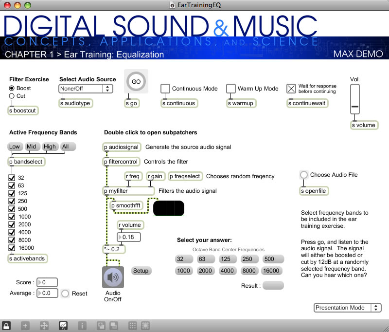
If you can’t afford Max, you might consider a free alternative, Pure Data, created by one of the originators of Max. Pure Data is open source software similar to Max in functionality and interface. For the Max programming exercises that involve audio programming, you might be able to use Pure Data and save yourself some money. However, PureData’s documentation is not nearly as comprehensive as the documentation for Max.
1.6.4 MATLAB and Octave

The icon shown in Figure 1.63 indicates there is a MATLAB exercise available for that section of the book. MATLAB (Figure 1.64) is a commercial mathematical modeling tool that allows you to experiment with digital sound at a low level of abstraction. MATLAB, which stands for “matrix lab,” is adept at manipulating matrices and arrays of data. Essentially, matrices are tables of information, and arrays are lists. Digital audio data related to a sound or piece of music is nothing more than an array of audio samples. The audio samples are generated in one of two basic ways in MATLAB. Sound can be recorded in an audio processing program like Adobe Audition, saved as an uncompressed PCM or a WAV file, and then input into MATLAB. Alternatively, it can be generated directly in MATLAB through the execution of sine functions. A sine function is given a frequency and amplitude related to the pitch and loudness of the desired sound. Executing a sine function at evenly spaced points produces numbers that constitute the audio data. Sine functions also can be added to each other to create complex sounds, the sound data can be plotted on a graph, and the sounds can be played in MATLAB. Operations on sine functions lay bare the mathematics of audio processing to give you a deeper understanding of filters, special effects, quantization error, dithering, and the like. Although such operations are embedded at a high level of abstraction in tools like Logic and Audition, MATLAB allows you to create them “by hand” so that you really understand how they work.
MATLAB also has extra toolkits that provide higher-level functions. For example, the signal processing toolkit gives you access to functions such as specialized waveform generators, transforms, frequency responses, impulse responses, FIR filters, IIR filters, and zero-pole diagram manipulations. The associated graphs help you to visualize how sound is changed when mathematical operations alter the properties of sound, amplitude, and phase.
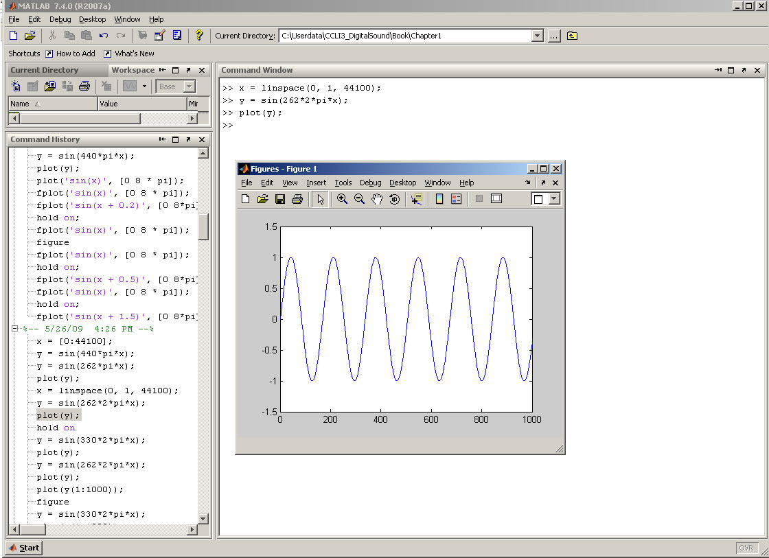
GNU Octave is an open source alternative to MATLAB that runs under the Linux, Unix, Mac OS X, or Windows operating systems. Like MATLAB, its specialty is array operations. Octave has most of the basic functionality of MATLAB, including the ability to read in or generate audio data, plot the data, perform basic array-based operations like adding or multiplying sine functions, and handle complex numbers. Octave doesn’t have the extensive signal processing toolbox that MATLAB offers. However, third-party extensions to Octave are freely downloadable on the web, and at least one third-party signal processing toolkit has been developed with filtering, windowing, and display functions.
1.6.5 C++ and Java Programming Exercises

[aside]Because the audio processing implemented in these exercises is done at a fairly low level of abstraction, the solutions we provide for the C++ programming exercises are written primarily in C, without emphasis on the object-oriented features of C++. For convenience, we use a few C++ constructs like dynamic memory allocation with new and variable declarations anywhere in the program.[/aside]
This book is intended to be useful not only to musicians, digital sound designers, and sound engineers, but also to computer scientists specializing in digital sound. Thus we include examples of sound processing done at a low level of abstraction, through C++ programs (Figure 1.65). The C++ programs that we use as examples are done on the Linux operating system. Linux is a good platform for audio programming because it is open-source, allowing you to have direct access to the sound card and operating system. Windows, in contrast, is much more of a black box. Thus, low-level sound programming is harder to do in this environment.
If you have access to a computer running under Linux, you probably already have a C++ compiler installed. If not, you can download and install a GNU compiler. You can also try our examples under Unix, a relative of Linux. Your computer and operating system dictate what header files need to be included in your programs, so you may need to check the documentation on this.
Some Java programming exercises are also included with this book. Java allows you to handle sound at a higher level of abstraction with packages such as java.sound.sampled and java.sound.midi. You’ll need a Java compiler and run-time to work with these programs.
1.7 Where to Go from Here
We’ve included lot of information in this section. Don’t worry if you don’t completely understand everything yet. As you go through each chapter, you’ll have the opportunity to experiment with all of these tools until you become confident with them. For now, start building up your workstation with the tools we’ve suggested, and enjoy the ride.
1.8 References
Franz, David. Recording and Producing in the Home Studio: A Complete Guide. Boston, MA: Berklee Press, 2004.
Kirn, Peter. Digital Audio: Industrial-Strength Production Techniques. Berkeley, CA: Peachpit Press, 2006.
Pohlmann, Ken C. The Compact Disc Handbook. Middleton, WI: A-R Editions, Inc., 1992.
Toole, Betty A. Ada, The Enchantress of Numbers. Mill Valley, CA: Strawberry Press, 1992.