Section 7.3.2 gives you algorithms for creating a variety of FIR filters. MATLAB also provides built-in functions for creating FIR and IIR filters. Let’s look at the IIR filters first.
MATLAB’s butter function creates an IIR filter called a Butterworth filter, named for its creator. Consider this sequence of commands:
N = 10;

f = 0.5;

[a,b] = butter(N, f);
The butter function call sends in two arguments: the order of the desired filter, N; and the and the cutoff frequency, f. The cutoff frequency is normalized so that the Nyquist frequency (½ the sampling rate) is 1, and all valid frequencies lie between 0 and 1. The function call returns two vectors, a and b, corresponding to the vectors a and b in Equation 7.4. (For a simple low-pass filter, an order of 6 is fine. The order is the number of coeffients.)
Now with the filter in hand, you can apply it using MATLAB’s filter function. The filter function takes the coefficients and the vector of audio samples as arguments:
output = filter(a,b,audio);
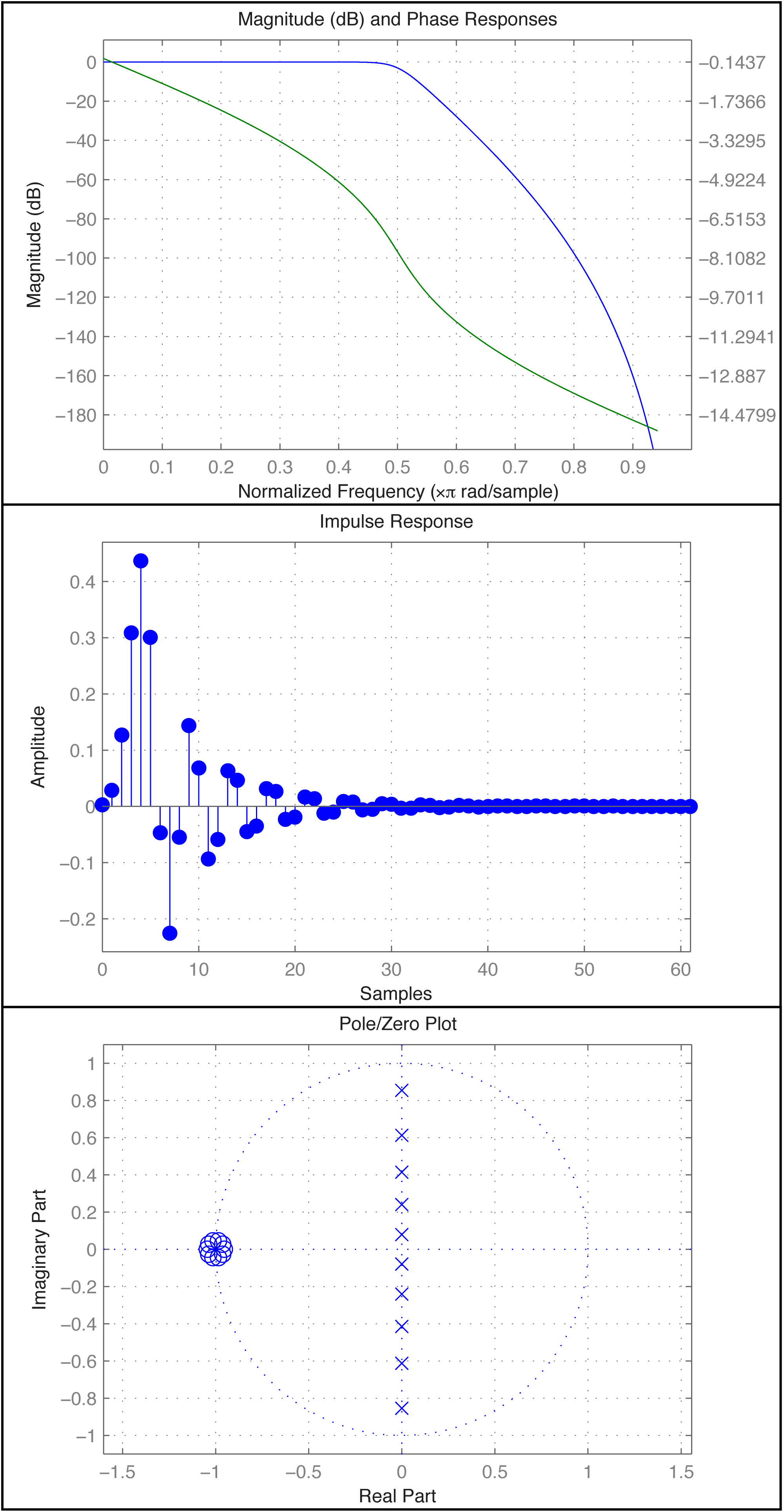
You can analyze the filter with the fvtool.
fvtool(a,b)
The fvtool provides a GUI through which you can see multiple views of the filter, including those in Figure 7.44. In the first figure, the blue line is the magnitude frequency response and the green line is phase.
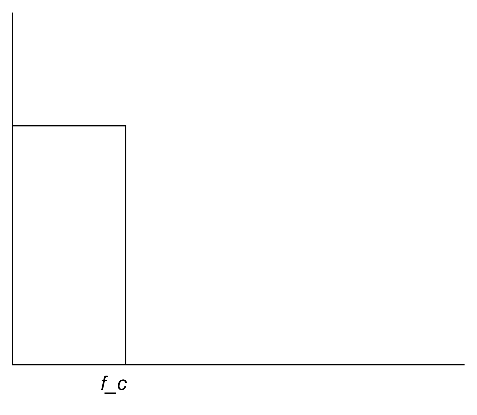
Another way to create and apply an IIR filter in MATLAB is by means of the function yulewalk. Let’s try a low-pass filter as a simple example. Figure 7.45 shows the idealized frequency response of a low-pass filter. The x-axis represents normalized frequencies, and f_c is the cutoff frequency. This particular filter allows frequencies that are up to ¼ the sampling rate to pass through, but filters out all the rest.
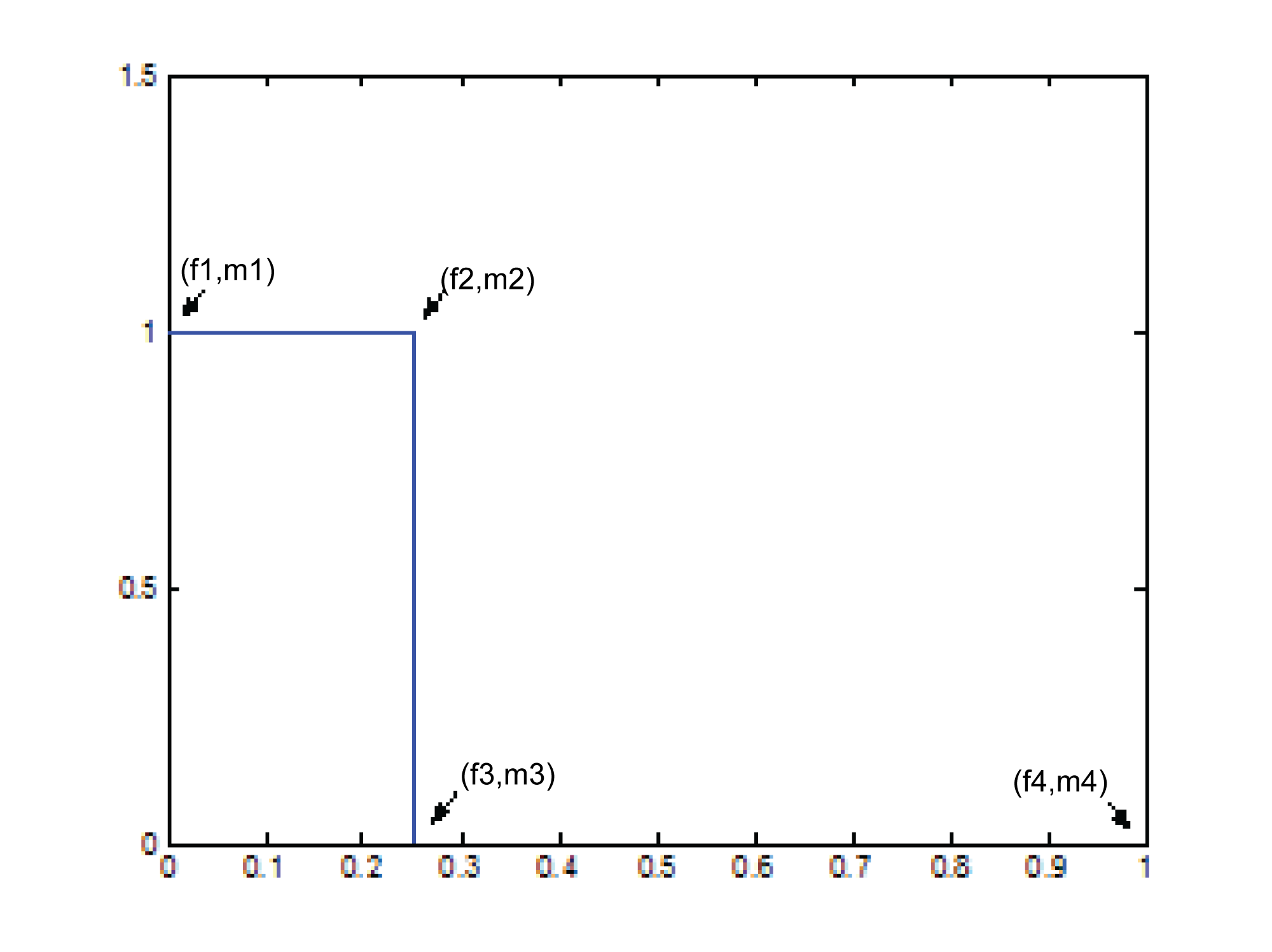
The first step in creating this filter is to store its “shape.” This information is stored in a pair of parallel vectors, which we’ll call f and m. For the four points on the graph in Figure 7.46, f stores the frequencies, and m stores the corresponding magnitudes. That is, $$\mathbf{f}=\left [ f1\; f2\; f3\; f4 \right ]$$ and $$\mathbf{m}=\left [ m1\; m2\; m3\; m4 \right ]$$, as illustrated in the figure. For the example filter we have
f = [0 0.25 0.25 1];

m = [1 1 0 0];
[aside]The yulewalk function in MATLAB is named for the Yule-Walker equations, a set of linear equations used in auto-regression modeling.[/aside]
Now that you have an ideal response, you use the yulewalk function in MATLAB to determine what coefficients to use to approximate the ideal response.
[a,b] = yulewalk(N,f,m)
Again, an order N=6 filter is sufficient for the low-pass filter. You can use the same filter function as above to apply the filter. The resulting filter is given in Figure 7.47. Clearly, the filter cannot be perfectly created, as you can see from the large ripple after the cutoff point.
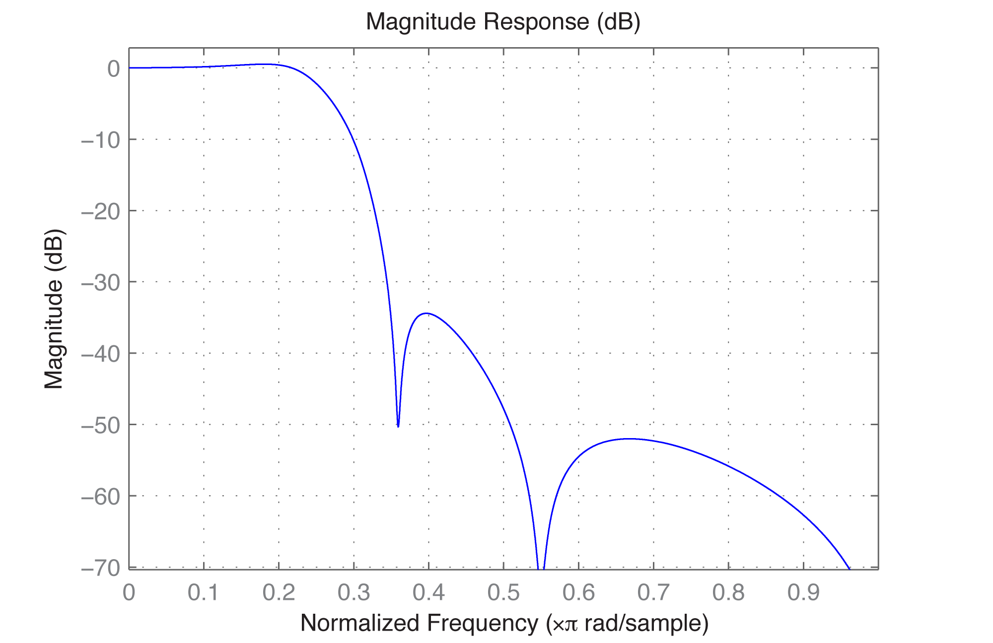
The finite counterpart to the yulewalk function is the fir2 function. Like butter, fir2 takes as input the order of the filter and two vectors corresponding to the shape of the filter’s frequency response. Thus, we can use the same f and m as before. fir2 returns the vector h constituting the filter.
h = fir2(N,f,m);
We need to use a higher order filter because this is an FIR. N=30 is probably high enough.
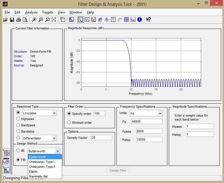
MATLAB’s extensive signal processing toolkit includes a Filter Designer with an easy-to-use graphical user interface that allows you to design the types of filters discussed in this chapter. A Butterworth filter is shown in Figure 7.48. You can adjust the parameters in the tool and see how the roll-off and ripples change accordingly. Experimenting with this tool helps you know what to expect from filters designed by different algorithms.