In Chapter 4, we discussed comb filtering in the context of acoustics and showed how comb filters can be made by means of delays. Let’s review comb filtering now.
A comb filter is created when two identical copies of a sound are summed (in the air, by means of computer processing, etc.), with one copy being offset in time from the other. The amount of offset determines which frequencies are combed out. The equation that predicts the combed frequency is given below.
[equation caption=”Equation 7.15 Comb filtering”]
$$!\begin{matrix}\textrm{Given a delay of }t\textrm{ seconds between two identical copies of a sound, then the frequencies of }f_{i}\textrm{ that will be combed are }\\ f_{i}=\frac{2i+1}{2t}\textrm{ for all integers }i\geq 0\end{matrix}$$
[/equation]
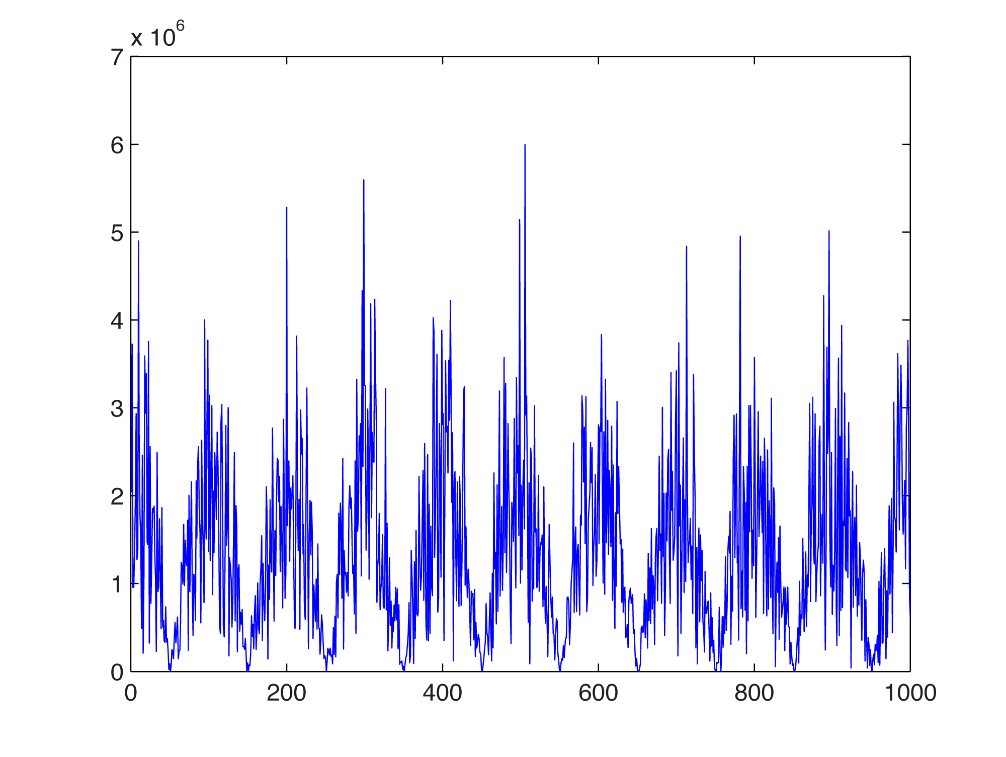
For a sampling rate of 44.1 kHz, 0.01 is equivalent to 441 samples. This delay is demonstrated in the MATLAB code below, which applies a delay of 0.01 seconds to white noise and graphs the resulting frequencies. (The white noise was created in Audition and saved in a raw PCM file.)
fid = fopen('WhiteNoise.pcm', 'r');

y = fread(fid, 'int16');

y = y(1:44100);

first = y(442:44100);

second = y(1:441);

y2 = cat(1, first, second);

y3 = y + y2;

plot(abs(fft(y3)));
You can see in Figure 7.42 that with a delay of 0.01 seconds, the frequencies that are combed out are 50 Hz, 150 Hz, 250 Hz, and so forth, while frequencies of 100 Hz, 200 Hz, 300 Hz, and so forth are boosted.
We created the comb filter above “by hand” by shifting the sample values and summing them. We can also use MATLAB’s fvtool.
a = [1  zeroes(1,440) 0.5];

b = [1];

fvtool(a,b);

axis([0 .008 -8 6]);

The x-axis in Figure 7.43 is normalized to the Nyquist frequency. That is, for a sampling rate of 44.1 kHz, the Nyquist frequency of 22,050 Hz is normalized to 1. Thus, 50 Hz falls at position 0.002 and 100 Hz at about 0.0045, etc.
Comb filters can be expressed as either non-recursive FIR filters or recursive IIR filters. A simple non-recursive comb filter is expressed by the following equation:
[equation caption=”Equation 7.16 Equation for an FIR comb filter”]
$$!\begin{matrix}\mathbf{y}\left ( n \right )=\mathbf{x}\left ( n \right )+g \ast \mathbf{x}\left ( n-m \right )\\\textit{where }\mathbf{y}\textit{ is the filtered audio in the time domain}\\\mathbf{x}\textit{ is the original audio in the time domain}\\m\textit{ is the amount of delay in samples, and}\left | g \right |\leq 1\end{matrix}$$
[/equation]
In an FIR comb filter, a fraction of an earlier sample is added to a later one, creating a repetition of the original sound. The distance between the two copies of the sound is controlled by m.
A simple recursive comb filter is expressed by the following equation:
[equation caption=”Equation 7.17 Equation for an IIR comb filter”]
$$!\begin{matrix}\mathbf{y}\left ( n \right )=\mathbf{x}\left ( n \right )+g \ast \mathbf{y}\left ( n-m \right )\\\textit{where }\mathbf{y}\textit{ is the filtered audio in the time domain}\\\mathbf{x}\textit{ is the original audio in the time domain}\\m\textit{ is the amount of delay in samples, and}\left | g \right |\leq 1\end{matrix}$$
[/equation]
You can see that Equation 7.17 represents a recursive filter because the output $$\mathbf{y}\left ( n-m \right )$$ is fed back in to create later output. With this feedback term, an earlier sound continues to have an effect on later sounds, but with decreasing intensity each time it is fed back in (because of the multiplier $$\left | g \right |\leq 1$$).