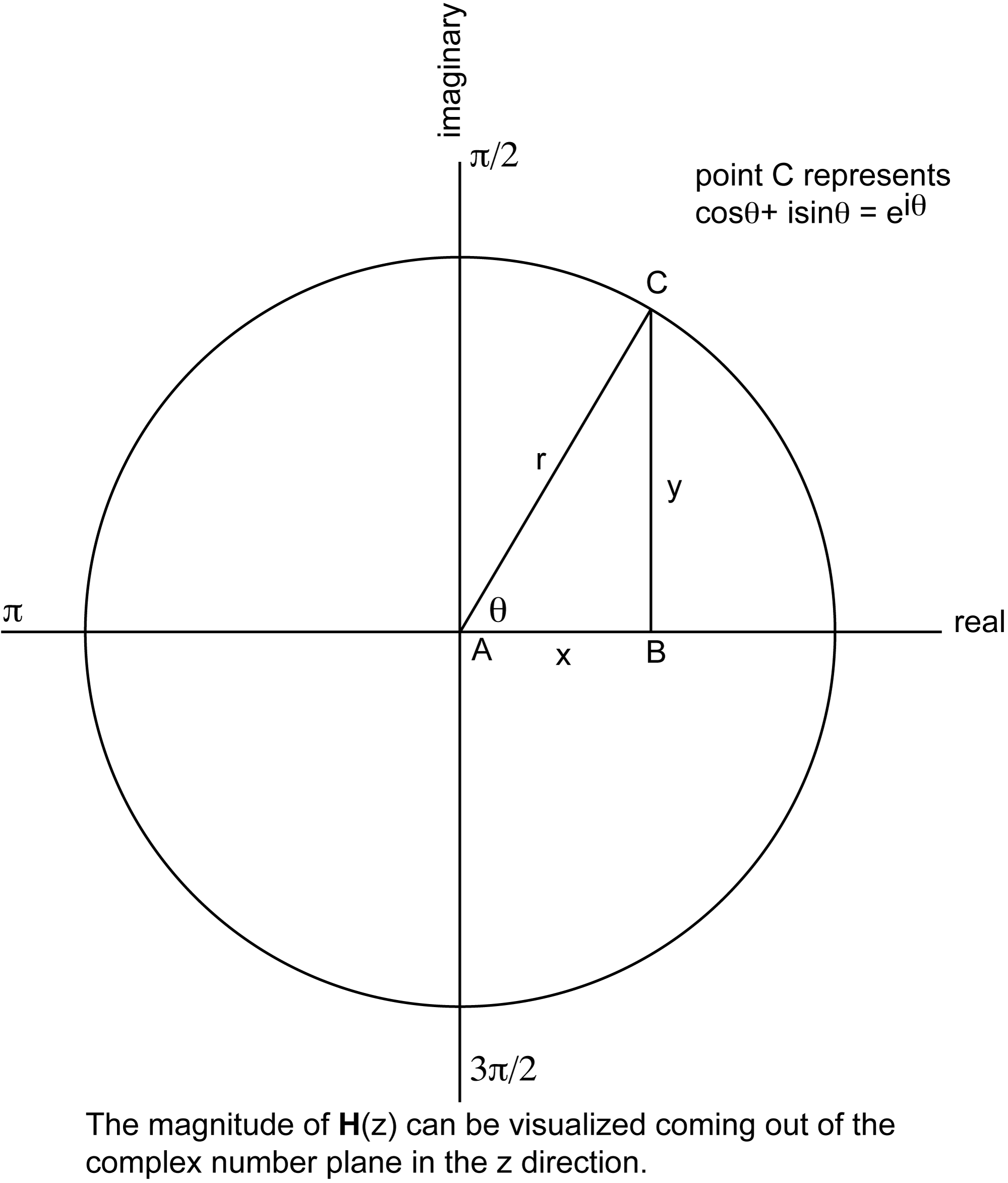
The function $$\mathbf{H}\left ( z \right )$$ defining a filter has a complex number z as its input parameter. Complex numbers are expressed as $$a+bi$$, where a is the real number component, b is the coefficient of the imaginary component, and i is $$\sqrt{-1}$$. The complex number plane can be graphed as shown in Figure 7.37, with the real component on the horizontal axis and the coefficient of the imaginary component on the vertical axis. Let’s look at how this works.
With regard to Figure 7.37, let x, y, and r denote the lengths of line segments $$\overline{AB}$$, $$\overline{BC}$$, and $$\overline{AC}$$ , respectively. Since the circle is a unit circle, $$r=1$$. From trigonometric relations, we get
$$!x=\cos \theta$$
$$!y=\sin \theta$$
Point C represents the number $$\cos \theta +i\sin \theta$$ on the complex number plane. By Euler’s identity, $$\cos \theta +i\sin \theta=e^{i\theta }$$. $$\mathbf{H}\left ( z \right )$$ is a function that is evaluated around the unit circle and graphed on the complex number plane. Since we are working with discrete values, we are evaluating the filter’s response at N discrete points evenly distributed around the unit circle. Specifically, the response for the $$k^{th}$$ frequency component is found by evaluating $$\mathbf{H}\left ( z_{k} \right )$$ at $$z=e^{i\theta }=e^{i\frac{2\pi k}{N}}$$ where N is the number of frequency components. The output, $$\mathbf{H}\left ( z_{k} \right )$$, is a complex number, but if you want to picture the output in the graph, you can consider only the magnitude of $$\mathbf{H}\left ( z_{k} \right )$$, which would be a real number coming out of the complex number plane (as we’ll show in Figure 7.41). This helps you to visualize how the filter attenuates or boosts the magnitudes of different frequency components.
This leads us to a description of the zero-pole diagram, a graph of a filter’s transfer function that marks places where the filter does the most or least attenuation (the zeroes and poles, as shown in Figure 7.38). As the numerator of $$\frac{\mathbf{Y}\left ( z \right )}{\mathbf{X}\left ( z \right )}$$ goes to 0, the output frequency is getting smaller relative to the input frequency. This is called a zero. As the denominator goes to 0, the output frequency is getting larger relative to the input frequency. This is called a pole.
To see the behavior of the filter, we can move around the unit circle looking at each frequency component at point $$e^{i\theta }$$ where $$\theta =\frac{2\pi k}{N}$$ for $$0\leq k< N-1$$. Let $$d_{zero}$$ be the point’s distance from a zero and $$d_{pole}$$ be the point’s distance from a pole. If, as you move from point $$P_{k}$$ to point $$P_{k+1}$$ (these points representing input frequencies $$e^{i\frac{2\pi k}{N}}$$ and $$e^{i\frac{2\pi\left ( k+1 \right )}{N}}$$ respectively), the ratio $$\frac{d_{zero}}{d_{pole}}$$ gets larger, then the filter is progressively allowing more of the frequency $$e^{i\frac{2\pi k}{N}}$$ to “pass through” as opposed to $$e^{i\frac{2\pi\left ( k+1 \right )}{N}}$$.
Let’s try this mathematically with a couple of examples. These examples will get you started in your understanding of zero-pole diagrams and the graphing of filters, but the subject is complex. MATLAB’s Help has more examples and more explanations, and you can find more details in the books on digital signal processing listed in our references.
First let’s try a simple FIR filter. The coefficients for this filter are . In the time domain, this filter can be seen as a convolution represented as follows:
[equation caption=”Equation 7.11 Convolution for a simple filter in the time domain”]
$$!\mathbf{y}\left ( n \right )=\sum_{k=0}^{1}\mathbf{h}\left ( k \right )\mathbf{x}\left ( n-k \right )=\mathbf{x}\left ( n \right )-0.5\mathbf{x}\left ( n-1 \right )$$
[/equation]
Converting the filter to the frequency domain by the z-transform, we get
[equation caption=”Equation 7.12 Delay filter represented as a transfer function”]
$$!\mathbf{H}\left ( z \right )=1-0.5z^{-1}=\frac{z\left ( 1-0.5z^{-1} \right )}{z}=\frac{z-0.5}{z}$$
[/equation]
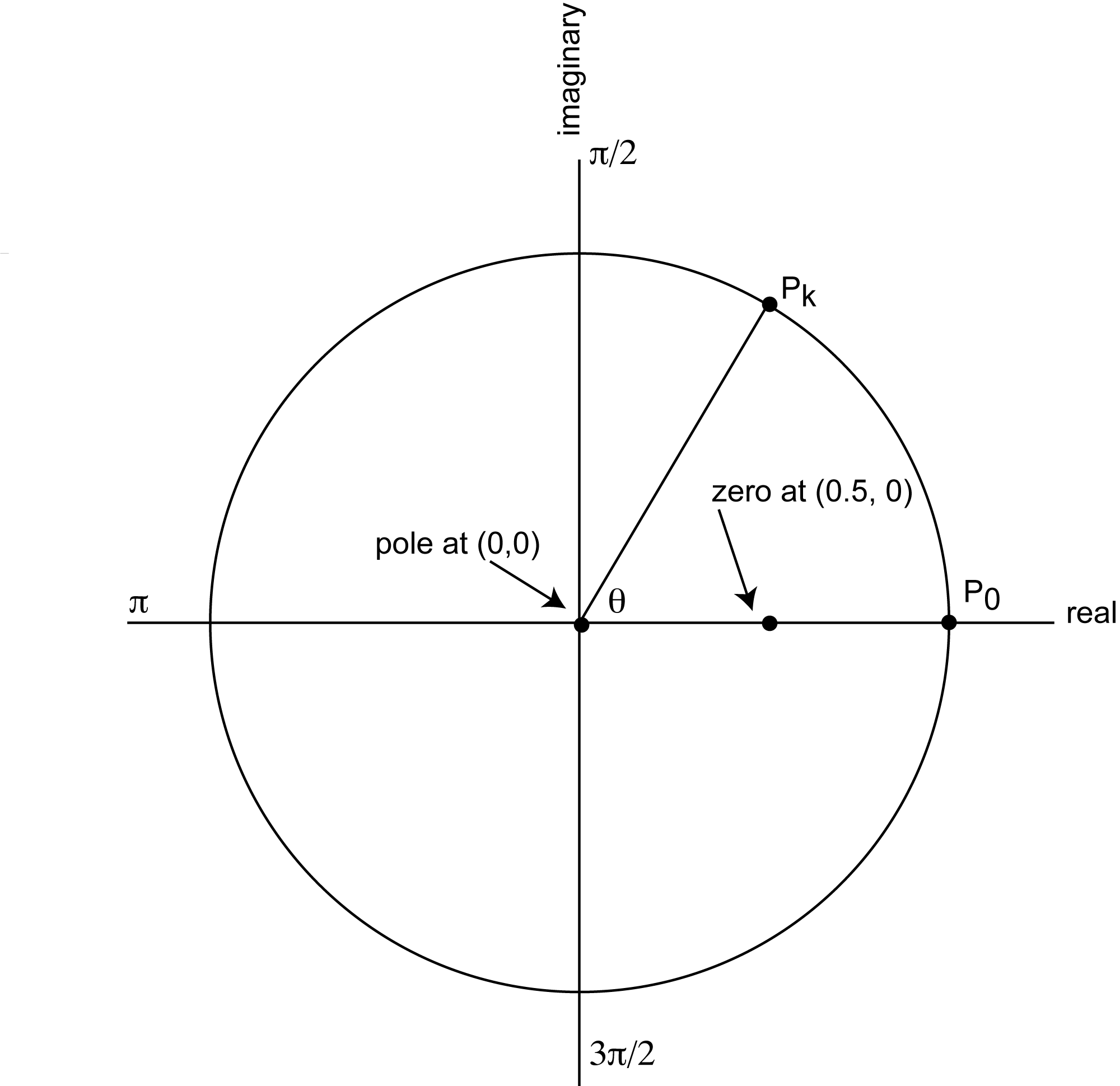
In the case of this simple filter, it’s easy to see where the zeroes and poles are. At $$z=0.5$$, the numerator is 0. Thus, a zero is at point (0.5, 0). At z = 0, the denominator is 0. Thus, a pole is at (0,0). There is no imaginary component to either the zero or the pole, so the coefficient of the imaginary part of the complex number is 0 in both cases.
Once we have the zeroes and poles, we can plot them on the graph representing the filter, $$\mathbf{H}\left ( z \right )$$, as shown in Figure 7.38. To analyze the filter’s effect on frequency components, consider the $$k^{th}$$ discrete point on the unit circle, point $$P_{k}$$, and the behavior of filter $$\mathbf{H}\left ( z \right )$$ at that point. Point $$P_{0}$$ is at the origin, and the angle formed between the x-axis and the line between $$P_{0}$$ and $$P_{k}$$is $$\theta =\frac{2\pi k}{N}$$. Each such point $$P_{k}$$ at angle $$\theta =\frac{2\pi k}{N}$$ corresponds to a frequency component $$e^{i}\frac{2\pi k}{N}$$ in the audio that is being filtered. Assume that the Nyquist frequency has been normalized to $$\pi$$. Thus, by the Nyquist theorem, the only valid frequency components to consider are between 0 and $$\pi$$. Let $$d_{zero}$$ be the distance between $$P_{k}$$ and a zero of the filter, and let $$d_{pole}$$ be the distance between $$P_{k}$$ and a pole. The magnitude of the frequency response, $$\mathbf{H}\left ( z \right )$$, will be smaller in proportion to $$\frac{d_{zero}}{d_{pole}}$$. For this example, the pole is at the origin so for all points $$P_{k}$$, $$d_{pole}$$ is 1. Thus, the magnitude of $$\frac{d_{zero}}{d_{pole}}$$ depends entirely on $$d_{zero}$$. As $$d_{zero}$$ gets larger, the frequency response gets larger. $$d_{zero}$$ increases as you move from $$\theta =0$$ to $$\theta =\pi$$. Since the frequency response increases as frequency increases, this filter is a high-pass filter, attenuating low frequencies more than high ones.
Now let’s try a simple IIR filter. Say that the equation for the filter is this:
[equation caption=”Equation 7.13 Equation for an IIR filter”]
$$!\mathbf{y}\left ( n \right )=\mathbf{x}\left ( n \right )-\mathbf{x}\left ( n-2 \right )-0.49\mathbf{y}\left ( n-2 \right )$$
[/equation]
The coefficients for the forward filter are $$\left [ 1,0,-1\right ]$$, and the coefficients for the feedback filter are $$\left [ 0, -0.49\right ]$$. Applying the transfer function form of the filter, we get
[equation caption=”Equation 7.14 Equation for IIR filter, version 2″]
$$!\mathbf{H}\left ( z \right )=\frac{1-z^{-2}}{1-0.49z^{-2}}=\frac{z^{2}-1}{z^{2}-0.49}=\frac{\left ( z+1 \right )\left ( z-1 \right )}{\left ( z+0.7i \right )\left ( z-0.7i \right )}$$
[/equation]
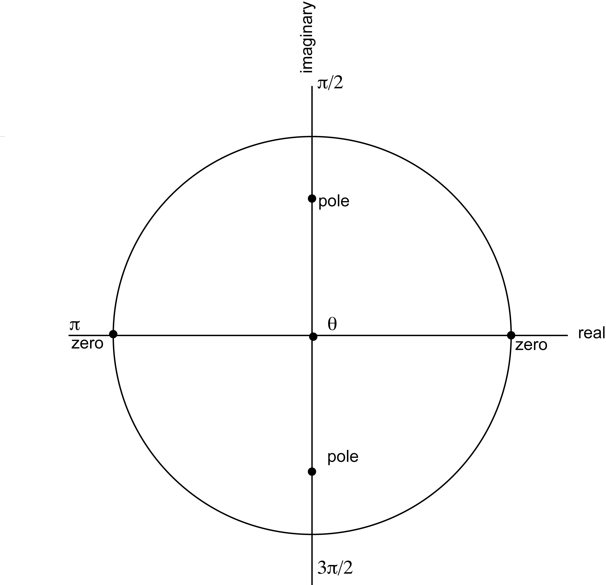
From Equation 7.14, we can see that there are zeroes at $$z=1$$ and $$z=-1$$ and poles at $$z=0.7i$$ and $$z=-0.7i$$. The zeroes and poles are plotted in Figure 7.39. This diagram is harder to analyze by inspection because there are two zeroes and two poles.
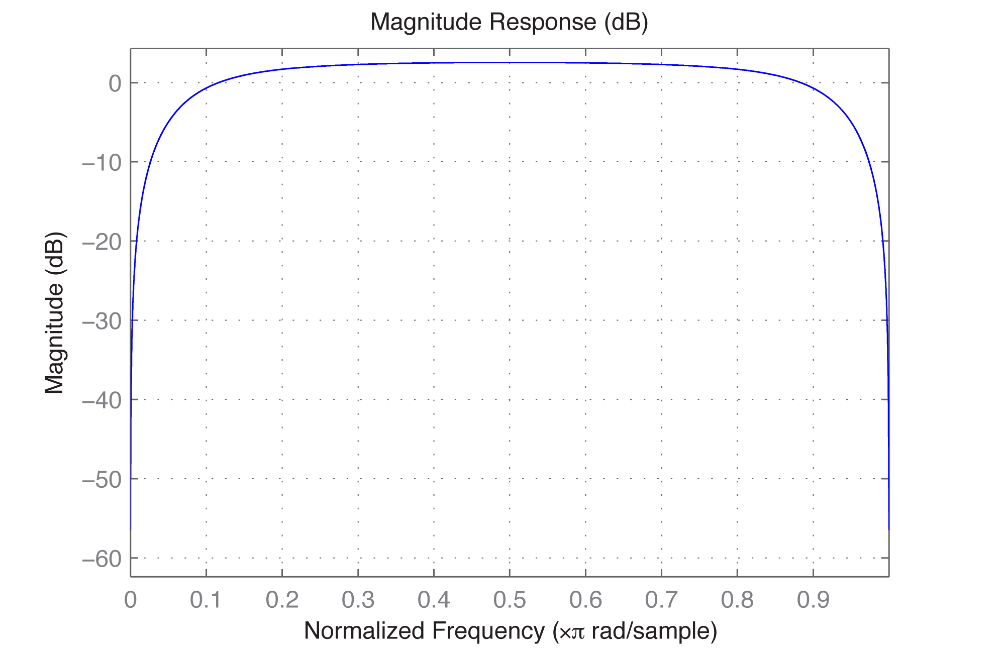
If we graph the frequency response of the filter, we can see that it’s a bandpass filter. We can do this with MATLAB’s fvtool (Filter Visualization Tool). The fvtool expects the coefficients of the transfer function (Equation 7.10) as arguments. The first argument of fvtool should be the coefficents of the numerator $$\left ( a_{0},a_{1},a_{2},\cdots \right )$$, and the second should be the coefficients of the denominator $$\left ( b_{1},b_{2},b_{3},\cdots \right )$$. Thus, the following MATLAB commands produce the graph of the frequency response, which shows that we have a bandpass filter with a rather wide band (Figure 7.40).
a = [1 0 -1];

b = [1 0 -0.49];

fvtool(a,b);
(You have to include the constant 1 as the first element of b.) MATLAB’s fvtool is discussed further in Section 7.3.9.
[wpfilebase tag=file id=167 tpl=supplement /]
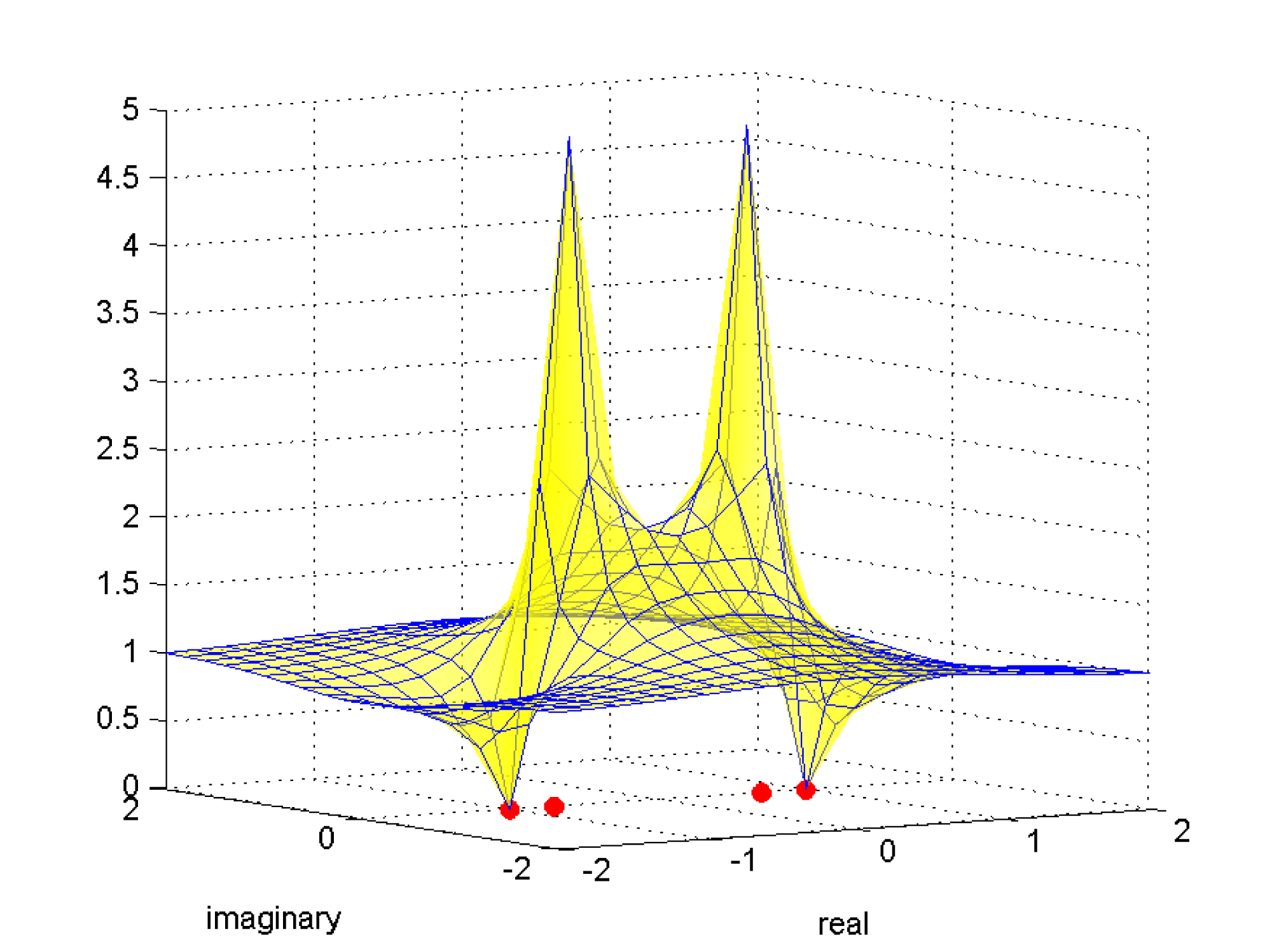
We can also graph the frequency response on the complex number plane, as we did with the zero-pole diagram, but this time we show the magnitude of the frequency response in the third dimension by means of a surface plot. This plot is shown in Figure 7.41. Writing a MATLAB function to create a graph such as this is left as an exercise.