In earlier chapters, we showed how audio signals can be represented in either the time domain or the frequency domain. In this section, you’ll see how mathematical operations are applied in these domains to implement filters, delays, reverberation, etc. Let’s start with the time domain.
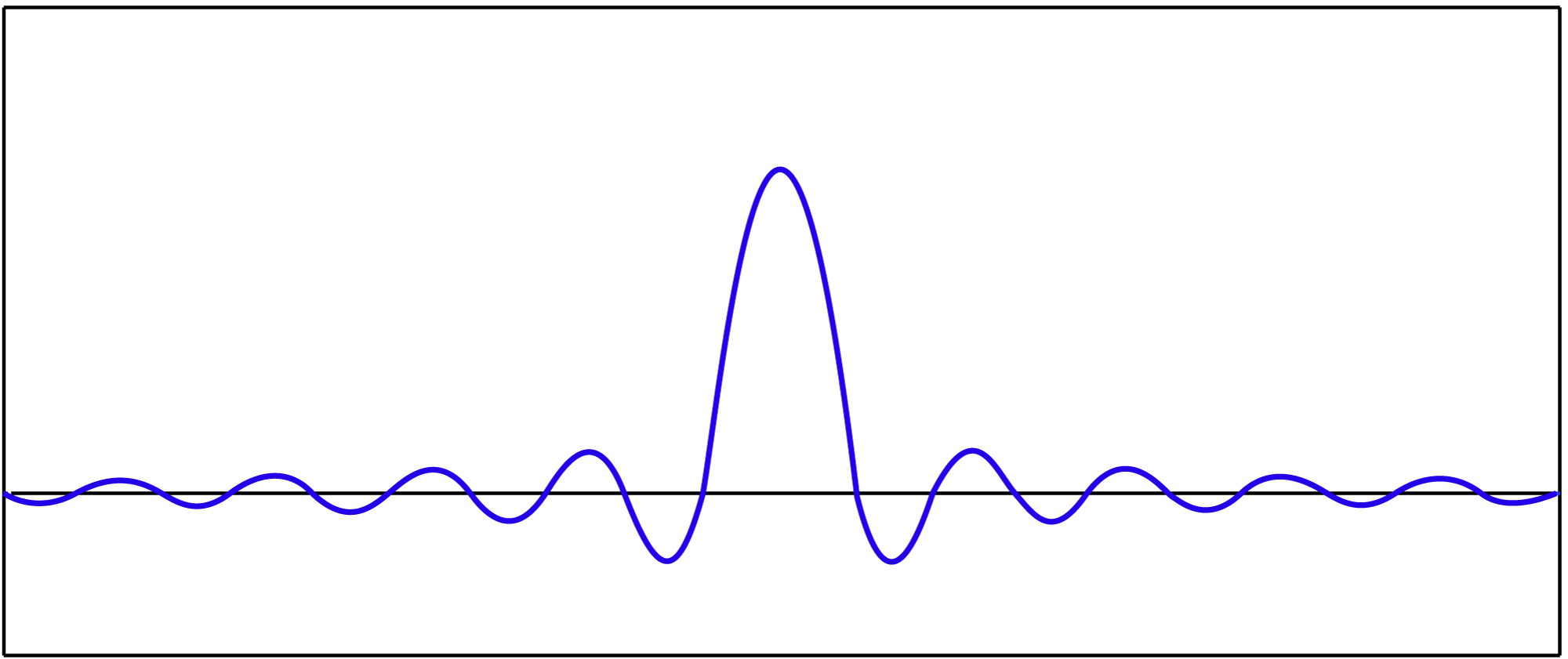
Filtering in the time domain is done by a convolution operation. Convolution uses a convolution filter, whichis an array of N values that, when graphed, takes the basic shape shown in Figure 7.32. A convolution filter is also referred to as a convolution mask, an impulse response (IR), or a convolution kernel. There are two commonly-used time-domain convolution filters that are applied to digital audio. They are FIR filters (finite impulse response) and IIR filters (infinite impulse response).
Equation 7.1 describes FIR filtering mathematically.
[equation caption=”Equation 7.1 FIR filter”]
$$!\begin{matrix}\mathbf{y}\left ( n \right )=\mathbf{h}\left ( n \right )\otimes \mathbf{x}\left ( n \right )=\sum_{k=0}^{N-1}\mathbf{h}\left ( k \right )\mathbf{x}\left ( n-k \right )=\sum_{k=0}^{N-1}\mathbf{a}_{k}\mathbf{x}\left ( n-k \right )\\\textit{where N is the size of the filter and}\: x\left ( n-k \right )=0\: if\; n-k< 0\end{matrix}$$
[/equation]
[aside]
You can actually think of equations such as Equation 7.1 in one of two ways: x and y could be understood as vectors of audio samples in the time domain, x being the input and y being the output. The equation must be executed N times to get each nth output sample. Alternatively, y could be understood as a function with input n. The function is executed N times to yield all N output samples.
[/aside]
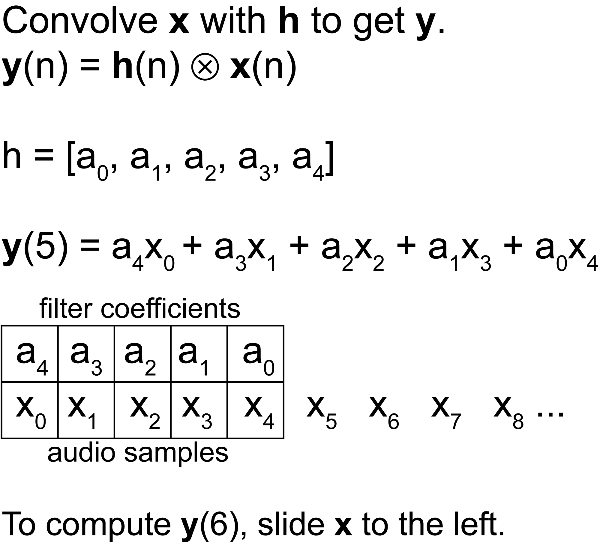
By our convention, boldface variables refer to vectors (i.e., arrays). In this equation, $$\mathbf{h}=\left [ a_{0},a_{1},a_{2}\cdots,a_{N-1} \right ]$$ is the convolution filter – which is a vector of multipliers to be applied successively to audio samples. The number of multipliers is the order of a filter, N in this case. N is sometimes also referred to as the number of taps in the filter.
It’s helpful to think of Equation 7.1 algorithmically, as described Algorithm 7.1. The notation $$\mathbf{y}\left ( n \right )$$ indicates that the $$n^{th}$$ output sample is created from a convolution of input values from the audio signal x and the filter multipliers in h, as given in the summation. The equation is repeated in a loop for every sample in the audio input.
[equation class=”algorithm” caption=”Algorithm 7.1 Convolution with a finite impulse response (FIR) filter”]
/*Input:
x, an array of digitized audio samples (i.e., in the time domain) of size M
h, a convolution filter of size N (Specifically, a finite-impulse-response filter, FIR
Output:
y, the audio samples, filtered
*/
for $$\left ( n=0\: to\; N-1 \right )$$ {
$$\mathbf{y}\left ( n \right )=\mathbf{h}\left ( n \right )\otimes \mathbf{x}\left ( n \right )=\sum_{k=0}^{N-1}\mathbf{h}\left ( k \right )\mathbf{x}\left ( n-k \right )$$
where $$x\left ( n-k \right )=0\: if\; n-k< 0$$
}
[/equation]
The FIR convolution process is described diagrammatically in Figure 7.33.
You can implement convolution yourself as a function, or you can use MATLAB’s conv function. The conv function requires two arguments. The first is an array containing the coefficients of the filter, and the second is the array of time domain audio samples to be convolved. Say that we have an FIR filter of size 3 defined as
[equation caption=”Equation 7.2 Equation for an example FIR filter”]
$$!y\left ( n \right )=0.4\left ( n \right )+0.3x\left ( n-1 \right )+0.3x(n-2)$$
[/equation]
In MATLAB, the coefficients of the filter can be stored in an array h like this:
h = [0.4 0.3 0.3];
Then we can read in a sound file and convolve it and listen to the results.
x = wavread('ToccataAndFugue.wav');

y = conv(h,x);

sound(y, 44100);
(This is just an arbitrary example with a random filter to demonstrate how you convolve in MATLAB. We haven’t yet considered how the filter itself is constructed.)
IIR filters are also time domain filters, but the process by which they work is a little different. An IIR filter has an infinite length, given by this equation:
[equation caption=”Equation 7.3 IIR Filter, infinite form”]
$$!\begin{matrix}\mathbf{y}\left ( n \right )=\mathbf{h}\left ( n \right )\otimes \mathbf{x}\left ( n \right )=\sum_{k=0}^{\infty }\mathbf{h}\left ( k \right )\mathbf{x}\left ( n-k \right )\\where\; x\left ( n-k \right )=0\: if\; n-k< 0\\\textit{and k is theoretically infinite}\end{matrix}$$
[/equation]
We can’t deal with an infinite summation in practice, but Equation 7.3 can be transformed to a difference equation form which gives us something we can work with.
[equation caption=”Equation 7.4 IIR filter, difference equation form”]
$$!\begin{matrix}\mathbf{y}\left ( n \right )=\mathbf{h}\left ( n \right )\otimes \mathbf{x}\left ( n \right )=\sum_{k=0}^{N-1}\mathbf{a}_{k}\mathbf{x}\left ( n-k \right )-\sum_{k=1}^{M}\mathbf{b}_{k}\mathbf{y}\left ( n-k \right )\\\textit{where N is the size of the forward filter, M is the size of the feedback filter, and}\; x\left ( n-k \right )=0\: if\; n-k< 0\end{matrix}$$
[/equation]
In Equation 7.4, N is the size (also called order) of the forward filter and M is the size of the feedback filter. The output from an IIR filter is determined by convolving the input and combining it with the feedback of previous output. In contrast, the output from an FIR filter is determined solely by convolving the input.
[wpfilebase tag=file id=156 tpl=supplement /]
FIR and IIR filters each have their advantages and disadvantages. In general, FIR filters require more memory and processor time. IIR filters can more efficiently create a sharp cutoff between frequencies that are filtered out and those that are not. An FIR filter requires a larger filter size to accomplish the same sharp cutoff as an IIR filter. IIR filters also have the advantage of having analog equivalents, which facilitates their design. An advantage of FIR filters is that they can be constrained to have linear phase response, which means that phase shifts for frequency components are proportional to the frequencies. This is good for filtering music because harmonic frequencies are phase-shifted by the same proportions, preserving their harmonic relationship. Another advantage of FIR filters is that they’re not as sensitive to the noise that results from low bit depth and round-off error.
The exercise associated with this section shows you how to make a convolution filter by recording an impulse response in an acoustical space. Also, in Section 7.3.9, we’ll show a way to apply an IIR filter in MATLAB.