6.3.3.1 Table-Lookup Oscillators and Wavetable Synthesis
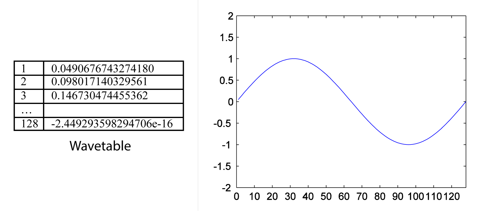
We have seen how single-frequency sound waves are easily generated by means of sinusoidal functions. In our example exercises, we’ve done this through computation, evaluating sine functions over time. In contrast, table-lookup oscillators generate waveforms by means of a set of look-up wavetables stored in contiguous memory locations. Each wavetable contains a list of sample values constituting one cycle of a sinusoidal wave, as illustrated in Figure 6.48. Multiple wavetables are stored so that waveforms of a wide range of frequencies can be generated.
[wpfilebase tag=file id=67 tpl=supplement /]
With a table-lookup oscillator, a waveform is created by advancing a pointer through a wavetable, reading the values, cycling back to the beginning of the table as necessary, and outputting the sound wave accordingly.
With a table of N samples representing one cycle of a waveform and an assumed sampling rate of r samples/s, you can generate a fundamental frequency of r/N Hz simply by reading the values out of the table at the sampling rate. This entails stepping through the indexes of the consecutive memory locations of the table. The wavetable in Figure 6.48 corresponds to a fundamental frequency of $$\frac{48000}{128}=375\: Hz$$.
Harmonics of the fundamental frequency of the wavetable can be created by skipping values or inserting extra values in between those in the table. For example, you can output a waveform with twice the frequency of the fundamental by reading out every other value in the table. You can output a waveform with ½ the frequency of the fundamental by reading each value twice, or by inserting values in between those in the table by interpolation.
The phase of the waveform can be varied by starting at an offset from the beginning of the wavetable. To start at a phase offset of $$p\pi $$ radians, you would start reading at index $$\frac{pN}{2}$$. For example, to start at an offset of π/2 in the wavetable of Figure 6.48, you would start at index $$\frac{\frac{1}{2}\ast 128}{2}=32$$.
To generate a waveform that is not a harmonic of the fundamental frequency, it’s necessary to add an increment to the consecutive indexes that are read out from the table. This increment i depends on the desired frequency f, the table length N, and the sampling rate r, defined by $$i=\frac{f\ast N}{r}$$. For example, to generate a waveform with frequency 750 Hz using the wavetable of Figure 6.48 and assuming a sampling rate of 48000 Hz, you would need an increment of $$i=\frac{750\ast 128}{48000}=2$$. We’ve chosen an example where the increment is an integer, which is good because the indexes into the table have to be integers.
What if you wanted a frequency of 390 Hz? Then the increment would be $$i=\frac{390\ast 128}{48000}=1.04$$, which is not an integer. In cases where the increment is not an integer, interpolation must be used. For example, if you want to go an increment of 1.04 from index 1, that would take you to index 2.04. Assuming that our wavetable is called table, you want a value equal to $$table\left [ 2 \right ]+0.04\ast \left ( table\left [ 3 \right ]-table\left [ 2 \right ] \right )$$. This is a rough way to do interpolation. Cubic spline interpolation can also be used as a better way of shaping the curve of the waveform. The exercise associated with this section suggests that you experiment with table-lookup oscillators in MATLAB.
[aside]The term “wavetable” is sometimes used to refer a memory bank of samples used by sound cards for MIDI sound generation. This can be misleading terminology, as wavetable synthesis is a different thing entirely.[/aside]
An extension of the use of table-lookup oscillators is wavetable synthesis. Wavetable synthesis was introduced in digital synthesizers in the 1970s by Wolfgang Palm in Germany. This was the era when the transition was being made from the analog to the digital realm. Wavetable synthesis uses multiple wavetables, combining them with additive synthesis and crossfading and shaping them with modulators, filters, and amplitude envelopes. The wavetables don’t necessarily have to represent simple sinusoidals but can be more complex waveforms. Wavetable synthesis was innovative in the 1970s in allowing for the creation of sounds not realizable with by solely analog means. This synthesis method has now evolved to the NWave-Waldorf synthesizer for the iPad.
6.3.3.2 Additive Synthesis
In Chapter 2, we introduced the concept of frequency components of complex waves. This is one of the most fundamental concepts in audio processing, dating back to the groundbreaking work of Jean-Baptiste Fourier in the early 1800s. Fourier was able to prove that any periodic waveform is composed of an infinite sum of single-frequency waveforms of varying frequencies and amplitudes. The single-frequency waveforms that are summed to make the more complex one are called the frequency components.
The implications of Fourier’s discovery are far reaching. It means that, theoretically, we can build whatever complex sounds we want just by adding sine waves. This is the basis of additive synthesis. We demonstrated how it worked in Chapter 2, illustrated by the production of square, sawtooth, and triangle waveforms. Additive synthesis of each of these waveforms begins with a sine wave of some fundamental frequency, f. As you recall, a square wave is constructed from an infinite sum of odd-numbered harmonics of f of diminishing amplitude, as in
$$!A\sin \left ( 2\pi ft \right )+\frac{A}{3}\sin \left ( 6\pi ft \right )+\frac{A}{5}\sin \left ( 10\pi ft \right )+\frac{A}{7}\sin \left ( 14\pi ft \right )+\frac{A}{9}\sin \left ( 18\pi ft \right )+\cdots$$
A sawtooth waveform can be constructed from an infinite sum of all harmonics of f of diminishing amplitude, as in
$$!\frac{2}{\pi }\left ( A\sin \left ( 2\pi ft \right )+\frac{A}{2}\sin \left ( 4\pi ft \right )+\frac{A}{3}\sin \left ( 6\pi ft \right )+\frac{A}{4}\sin \left ( 8\pi ft \right )+\frac{A}{5}\sin \left ( 10\pi ft \right )+\cdots \right )$$
A triangle waveform can be constructed from an infinite sum of odd-numbered harmonics of f that diminish in amplitude and vary in their sign, as in
$$!\frac{8}{\pi^{2} }\left ( A\sin \left ( 2\pi ft \right )+\frac{A}{3^{2}}\sin \left ( 6\pi ft \right )+\frac{A}{5^{2}}\sin \left ( 10\pi ft \right )-\frac{A}{7^{2}}\sin \left ( 14\pi ft \right )+\frac{A}{9^{2}}\sin \left ( 18\pi ft \right )-\frac{A}{11^{2}}\sin \left ( 22\pi ft \right )+\cdots \right )$$
These basic waveforms turn out to be very important in subtractive synthesis, as they serve as a starting point from which other more complex sounds can be created.
To be able to create a sound by additive synthesis, you need to know the frequency components to add together. It’s usually difficult to get the sound you want by adding waveforms from the ground up. In turns out that subtractive synthesis is often an easier way to proceed.
6.3.3.3 Subtractive Synthesis
The first synthesizers, including the Moog and Buchla’s Music Box, were analog synthesizers that made distinctive electronic sounds different from what is produced by traditional instruments. This was part of the fascination that listeners had for them. They did this by subtractive synthesis, a process that begins with a basic sound and then selectively removes frequency components. The first digital synthesizers imitated their analog precursors. Thus, when people speak of “analog synthesizers” today, they often mean digital subtractive synthesizers. The Subtractor Polyphonic Synthesizer shown in Figure 6.19 is an example of one of these.
The development of subtractive synthesis arose from an analysis of musical instruments and the way they create their sound, the human voice being among those instruments. Such sounds can be divided into two components: a source of excitation and a resonator. For a violin, the source is the bow being drawn across the string, and the resonator is the body of the violin. For the human voice, the source results from air movement and muscle contractions of the vocal chords, and the resonator is the mouth. In a subtractive synthesizer, the source could be a pulse, sawtooth, or triangle wave or random noise of different colors (colors corresponding to how the noise is spread out over the frequency spectrum). Frequently, preset patches are provided, which are basic waveforms with certain settings like amplitude envelopes already applied (another usage of the term patch). Filters are provided that allow you to remove selected frequency components. For example, you could start with a sawtooth wave and filter out some of the higher harmonic frequencies, creating something that sounds fairly similar to a stringed instrument. An amplitude envelope could be applied also to shape the attack, decay, sustain, and release of the sound.
The exercise suggests that you experiment with subtractive synthesis in C++ by beginning with a waveform, subtracting some of its frequency components, and applying an envelope.
6.3.3.4 Amplitude Modulation (AM)
Amplitude, phase, and frequency modulation are three types of modulation that can be applied to synthesize sounds in a digital synthesizer. We explain the mathematical operations below. In Section 0, we defined modulation as the process of changing the shape of a waveform over time. Modulation has long been used in analog telecommunication systems as a way to transmit a signal on a fixed frequency channel. The frequency on which a television or radio station is broadcast is referred to as the carrier signal and the message “written on” the carrier is called the modulator signal. The message can be encoded on the carrier signal in one of three ways: AM (amplitude modulation), PM (phase modulation), or FM (frequency modulation).
Amplitude modulation (AM) is commonly used in radio transmissions. It entails sending a message by modulating the amplitude of a carrier signal with a modulator signal.
In the realm of digital sound as created by synthesizers, AM can be used to generate a digital audio signal of N samples by application of the following equation:
[equation caption=”Equation 6.1 Amplitude modulation for digital synthesis”]
$$!a\left ( n \right )=\sin \left ( \omega _{c}n/r \right )\ast \left ( 1.0+A\cos\left ( \omega _{m}n/r \right ) \right )$$
for $$0\leq n\leq N-1$$
where N is the number of samples,
$$\omega _{c}$$ is the angular frequency of the carrier signal
$$\omega _{m}$$ is the angular frequency of the modulator signal
r is the sampling rate
and A is the amplitude
[/equation]
The process is expressed algorithmically in Algorithm 6.8. The algorithm shows that the AM synthesis equation must be applied to generate each of the samples for $$1\leq t\leq N$$.
[equation class=”algorithm” caption=”Algorithm 6.1 Amplitude modulation for digital synthesis”]
algorithm amplitude_modulation
/*
Input:
f_c, the frequency of the carrier signal
f_m, the frequency of a low frequency modulator signal
N, the number of samples you want to create
r, the sampling rate
A, to adjust the amplitude of the
Output:
y, an array of audio samples where the carrier has been amplitude modulated by the modulator */
{
	for (n = 1 to N)
		y[n] = sin(2*pi*f_c*n/r) * (1.0 + A*cos(2*pi*f_m*n/r));
}
[/equation]
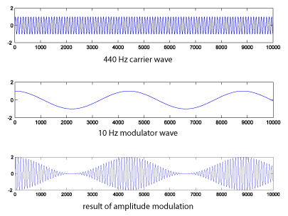
Algorithm 6.1 can be executed at the MATLAB command line with the statements below, generating the graphs is Figure 6.49. Because MATLAB executes the statements as vector operations, a loop is not required. (Alternatively, a MATLAB program could be written using a loop.) For simplicity, we’ll assume $$A=1$$ in what follows.
N = 44100;
r = 44100;
n = [1:N];
f_m = 10;
f_c = 440;
m = cos(2*pi*f_m*n/r);
c = sin(2*pi*f_c*n/r);
figure;
AM = c.*(1.0 + m);
plot(m(1:10000));
axis([0 10000 -2 2]);
figure;
plot(c(1:10000));
axis([0 10000 -2 2]);
figure;
plot(AM(1:10000));
axis([0 10000 -2 2]);
sound(c, 44100);
sound(m, 44100);
sound(AM, 44100);
This yields the following graphs:

If you listen to the result, you’ll see that amplitude modulation creates a kind of tremolo effect.
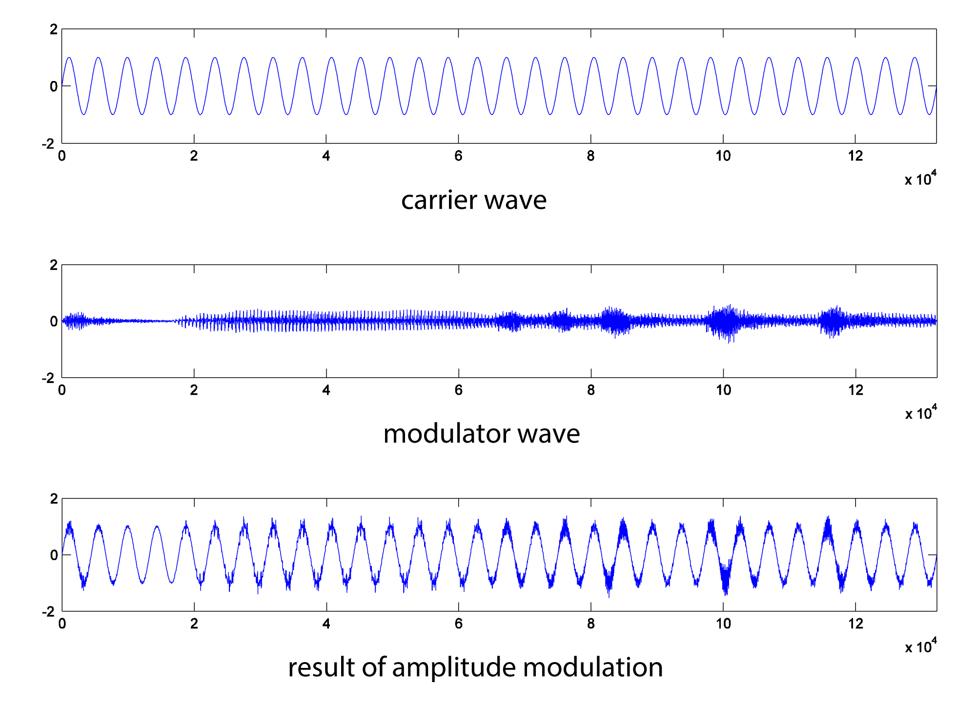
The same process can be accomplished with more complex waveforms. HornsE04.wav is a 132,300-sample audio clip of horns playing, at a sampling rate of 44,100 Hz. Below, we shape it with a 440 Hz cosine wave (Figure 6.50).
N = 132300;
r = 44100;
c = audioread('HornsE04.wav');
n = [1:N];
m = sin(2*pi*10*n/r);
m = transpose(m);
AM2 = c .* (1.0 + m);
figure;
plot(c);
axis([0 132300 -2 2]);
figure;
plot(m);
axis([0 132300 -2 2]);
figure;
plot(AM2);
axis([0 132300 -2 2]);
sound(c, 44100);
sound(m, 44100);
sound(AM2, 44100);
The audio effect is different, depending on which signal is chosen as the carrier and which as the modulator. Below, the carrier and modulator are reversed from the previous example, generating the graphs in Figure 6.51.
N = 132300;
r = 44100;
m = audioread('HornsE04.wav');
n = [1:N];
c = sin(2*pi*10*n/r);
c = transpose(c);
AM3 = c .* (1.0 + m);
figure;
plot(c);
axis([0 132300 -2 2]);
figure;
plot(m);
axis([0 132300 -2 2]);
figure;
plot(AM3);
axis([0 132300 -2 2]);
sound(c, 44100);
sound(m, 44100);
sound(AM3, 44100);
Amplitude modulation produces new frequency components in the resulting waveform at $$f_{c}+f_{m}$$ and $$f_{c}-f_{m}$$, where $$f_{c}$$ is the frequency of the carrier and $$f_{m}$$ is the frequency of the modulator. These are called sidebands. You can verify that the sidebands are at $$f_{c}+f_{m}$$ and $$f_{c}-f_{m}$$with a little math based on the properties of sines and cosines.
$$!\cos \left ( 2\pi f_{c}n \right )\left ( 1.0+\cos \left ( 2\pi f_{m}n \right ) \right )=\cos \left ( 2\pi f_{c}n \right )+\cos \left ( 2\pi f_{c}n \right )\cos \left ( 2\pi f_{m}n \right )=\cos \left ( 2\pi f_{c}n \right )+\frac{1}{2}\cos \left ( 2\pi \left ( f_{c}+f_{m} \right )n \right )+\frac{1}{2}\cos \left ( 2\pi \left ( f_{c}-f_{m} \right )n \right )$$
(The third step comes from the cosine product rule.) This derivation shows that there are three frequency components: one with frequency $$f_{c}$$, a second with frequency $$f_{c}+f_{m}$$, and a third with frequency $$f_{c}-f_{m}$$.
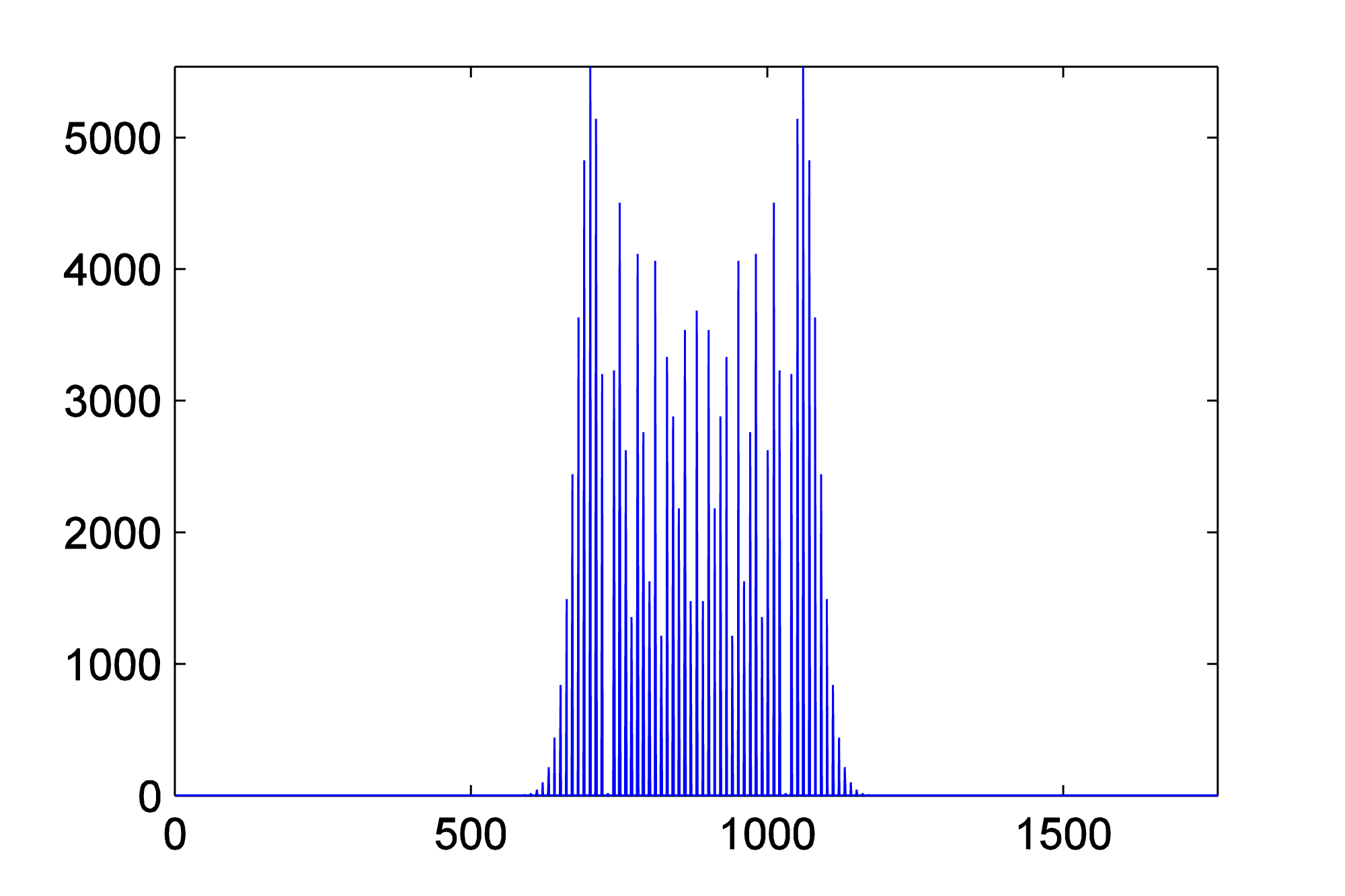
To verify this with an example, you can generate a graph of the sidebands in MATLAB by doing a Fourier transfer of the waveform generated by AM and plotting the magnitudes of the frequency components. MATLAB’s fft function does a Fourier transform of a vector of audio data, returning a vector of complex numbers. The abs function turns the complex numbers into a vector of magnitudes of frequency components. Then these values can be plotted with the plot function. We show the graph only from frequencies 1 through 600 Hz, since the only frequency components for this example lie in this range. Figure 6.52 shows the sidebands corresponding the AM performed in Figure 6.49. The sidebands are at 450 Hz and 460 Hz, as predicted.
figure;
fftmag = abs(fft(AM));
plot(fftmag(1:600));
6.3.3.5 Ring Modulation
Ring modulation entails simply multiplying two signals. To create a digital signal using ring modulation, the Equation 6.2 can be applied.
[equation caption=”Equation 6.2 Ring modulation for digital synthesis”]
$$r\left ( n \right )=A_{1}\sin \left ( \omega _{1}n/r \right )\ast A_{2}\sin \left ( \omega _{2}n/r \right )$$
for $$0\leq n\leq N-1$$
where N is the number of samples,
r is the sampling rate,
where $$\omega _{1}$$ and $$\omega _{2}$$ are the angular frequencies of two signals, and $$A _{1}$$ and $$A _{2}$$ are their respective amplitudes
[/equation]
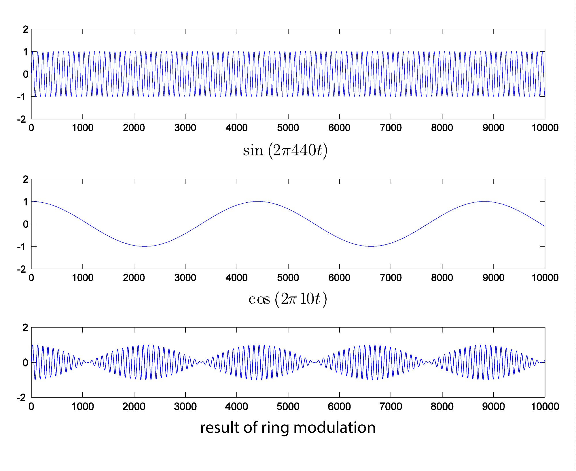
Since multiplication is commutative, there’s no sense in which one signal is the carrier and the other the modulator. Ring modulation is illustrated with two simple sine waves in Figure 6.53. The ring modulated waveform is generated with the MATLAB commands below. Again, we set amplitudes to 1.
N = 44100;
r = 44100;
n = [1:N];
w1 = 440;
w2 = 10;
rm = sin(2*pi*w1*n/r) .* cos(2*pi*w2*n/r);
plot(rm(1:10000));
axis([1 10000 -2 2]);
6.3.3.6 Phase Modulation (PM)
Even more interesting audio effects can be created with phase (PM) and frequency modulation (FM). We’re all familiar with FM radio, which is based on sending a signal by frequency modulation. Phase modulation is not used extensively in radio transmissions because it can be ambiguous to interpret at the receiving end, but it turns out to be fairly easy to implement PM in digital synthesizers. Some hardware-based synthesizers that are commonly referred to as FM actually use PM synthesis internally – the Yamaha DX series, for example.
Recall that the general equation for a cosine waveform is $$A\cos \left ( 2\pi fn+\phi \right )$$ where f is the frequency and $$\phi$$ is the phase. Phase modulation involves changing the phase over time. Equation 6.3 uses phase modulation to generate a digital signal.
[equation caption=”Equation 6.3 Phase modulation for digital synthesis”]
$$p\left ( t \right )=A\cos \left ( \omega _{c}n/r+I\sin \left ( \omega _{m}n/r \right ) \right )$$
for $$0\leq n\leq N-1$$
where N is the number of samples,
$$\omega _{c}$$ is the angular frequency of the carrier signal,
$$\omega _{m}$$ is the angular frequency of the modulator signal,
r is the sampling rate
I is the index of modulation
and A is the amplitude
[/equation]
Phase modulation is demonstrated in MATLAB with the following statements:
N = 44100;
r = 44100;
n = [1:N];
f_m = 10;
f_c = 440;
w_m = 2 * pi * f_m;
w_c = 2 * pi * f_c;
A = 1;
I = 1;
p = A*cos(w_c * n/r + I*sin(w_m * n/r));
plot(p);
axis([1 30000 -2 2]);
sound(p, 44100);
The result is graphed in Figure 6.54.
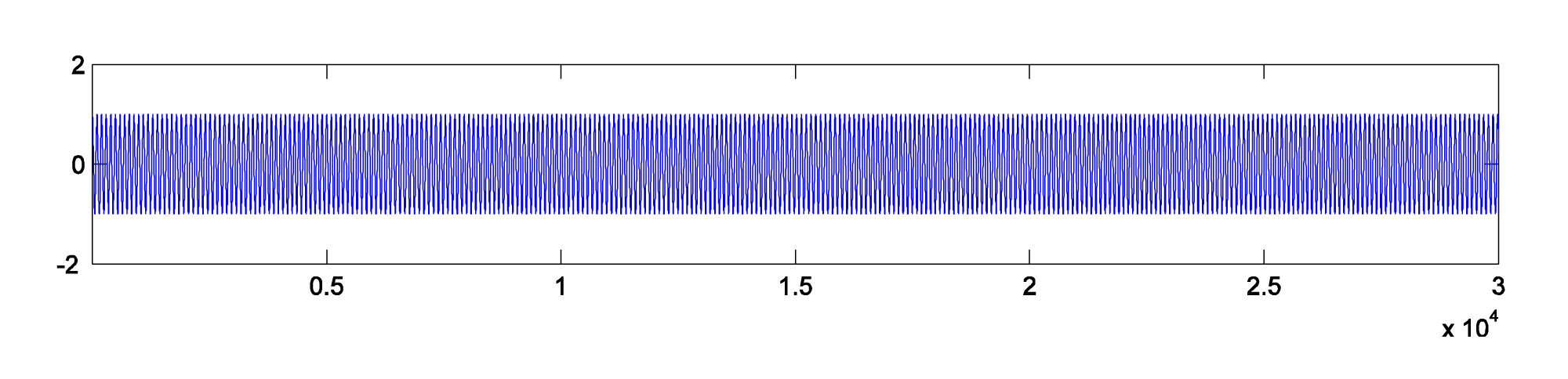
Figure 6.54 Phase modulation using two sinusoidals, where $$\omega _{c}=2\pi 440$$ and $$\omega _{m}=2\pi 10$$
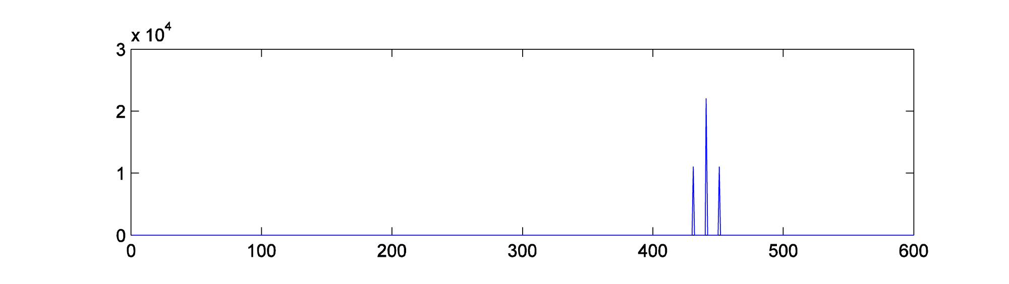
The frequency components shown in Figure 6.55 are plotted in MATLAB with
fp = fft2(p);
figure;
plot(abs(fp));
axis([400 480 0 18000]);
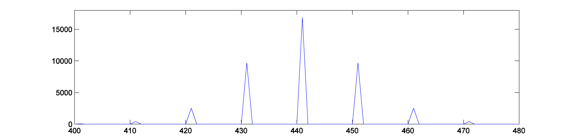
Phase modulation produces an infinite number of sidebands (many of whose amplitudes are too small to be detected). This fact is expressed in Equation 6.4.
[equation caption=”Equation 6.4 Phase modulation equivalence with additive synthesis”]
$$!\cos \left ( \omega _{c}n+I\sin \left ( \omega _{m}n \right ) \right )=\sum_{k=-\infty }^{\infty }J_{k}\left ( I \right )\cos \left ( \left [ \omega _{c}+k\omega _{m} \right ]n \right )$$
[/equation]
$$J_{k}\left ( I \right )$$ gives the amplitude of the frequency component for each kth component in the phase-modulated signal. These scaling functions $$J_{k}\left ( I \right )$$ are called Bessel functions of the first kind. It’s beyond the scope of the book to define these functions further. You can experiment for yourself to see that the frequency components have amplitudes that depend on I. If you listen to the sounds created, you’ll find that the timbres of the sounds can also be caused to change over time by changing I. The frequencies of the components, on the other hand, depend on the ratio of $$\omega _{c}/\omega _{m}$$. You can try varying the MATLAB commands above to experience the wide variety of sounds that can be created with phase modulation. You should also consider the possibilities of applying additive or subtractive synthesis to multiple phase-modulated waveforms.
The solution to the exercise associated with the next section gives a MATLAB .m program for phase modulation.
6.3.3.7 Frequency Modulation (FM)
We have seen in the previous section that phase modulation can be applied to the digital synthesis of a wide variety of waveforms. Frequency modulation is equally versatile and frequently used in digital synthesizers. Frequency modulation is defined recursively as follows:
[equation caption=”Equation 6.5 Frequency modulation for digital synthesis”]
$$f\left ( n \right )=A\cos \left ( p\left ( n \right ) \right )$$ and
$$p\left ( n \right )=p\left ( n-1 \right )+\frac{\omega _{c}}{r}+\left ( \frac{I\omega _{m}}{r}\ast \cos \left ( \frac{n\ast \omega _{m}}{r} \right ) \right )$$,
for $$1\leq n\leq N-1$$, and
$$p\left ( 0 \right )=\frac{\omega _{c}}{r}+ \frac{I\omega _{m}}{r}$$,
where N is the number of samples,
$$\omega_{c}$$ is the angular frequency of the carrier signal,
$$\omega_{m}$$ is the angular frequency of the modulator signal,
r is the sampling rate,
I is the index of modulation,
and A is amplitude
[/equation]
[wpfilebase tag=file id=69 tpl=supplement /]
Frequency modulation can yield results identical to phase modulation, depending on how inputs parameters are handled in the implementation. A difference between phase and frequency modulation is the perspective from which the modulation is handled. Obviously, the former is shaping a waveform by modulating the phase, while the latter is modulating the frequency. In frequency modulation, the change in the frequency can be handled by a parameter d, an absolute change in carrier signal frequency, which is defined by $$d=If_{m}$$. The input parameters $$N=44100$$, $$r=4100$$, $$f_{c}=880$$, $$f_{m}=10$$, $$A=1$$, and $$d=100$$ yield the graphs shown in Figure 6.56 and Figure 6.57. We suggest that you try to replicate these results by writing a MATLAB program based on Equation 6.5 defining frequency modulation.
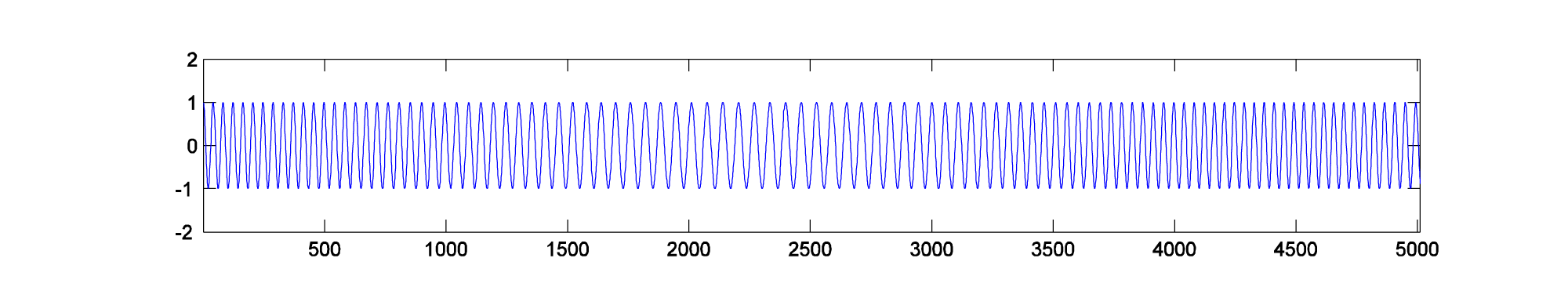
Figure 6.56 Frequency modulation using two sinusoidals, where $$\omega _{c}=2\pi 880$$ and $$\omega _{m}=2\pi 10$$