5.3.7 The Mathematics of Dithering and Noise Shaping

[wpfilebase tag=file id=97 tpl=supplement /]

[wpfilebase tag=file id=61 tpl=supplement /]

Dithering is described in Section 5.1.2.5 as the addition of low-amplitude random noise to an audio signal as it is being quantized. The purpose of dithering is to prevent neighboring sample values from quantizing all to the same level, which can cause breaks or choppiness in the sound.   Noise shaping can be performed in conjunction with dithering to raise the noise to a higher frequency where it is not noticed as much. Now let’s look at the mathematics of dithering and noise shaping.

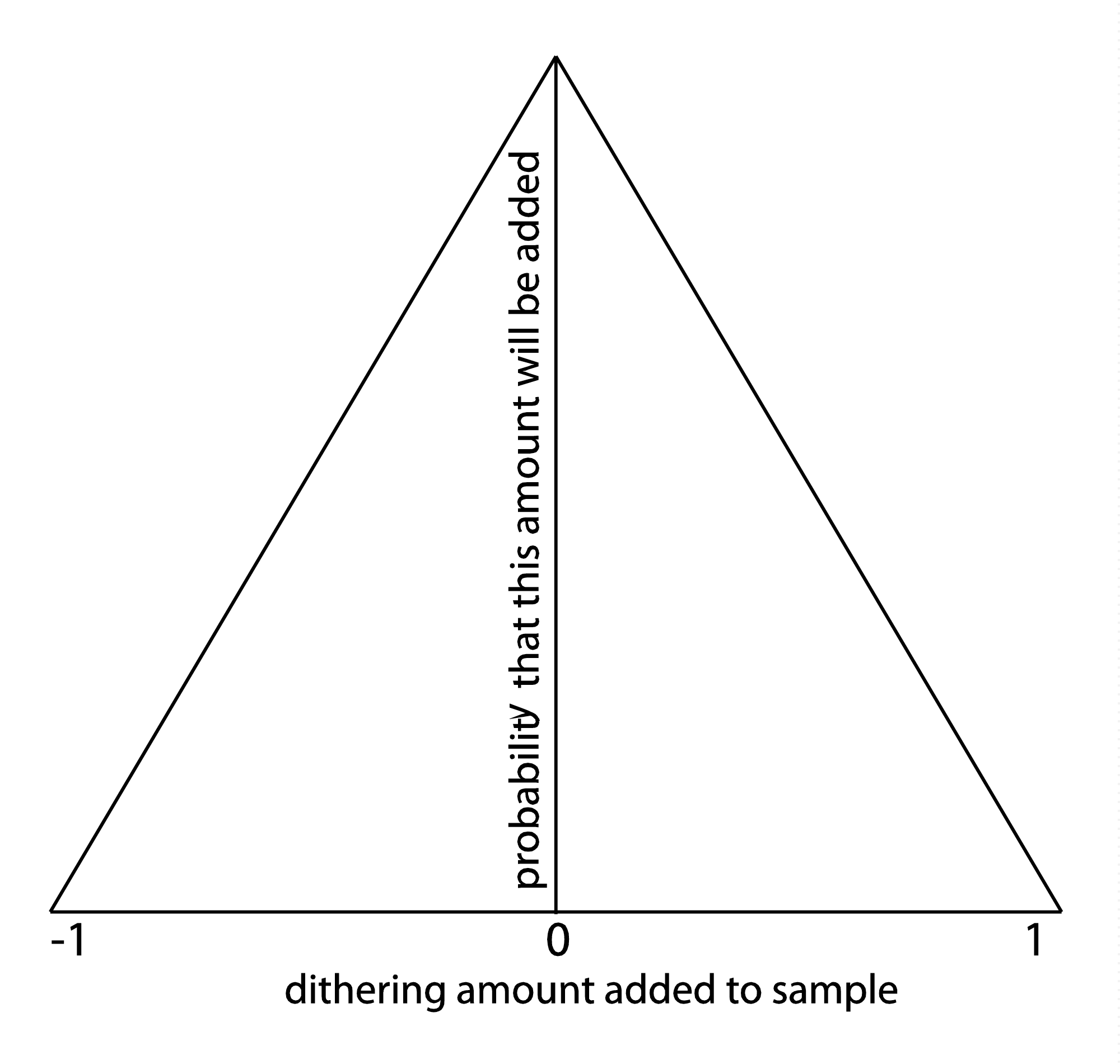
First, the amount of random noise to be added to each sample must be determined. A probability density function can be used for this purpose. We’ll use the triangular probability density function graphed in Figure 5.39 as an example. This graph depicts the following:

• There is 0 probability that an amount less than -1 and greater than 1 will be added to any given sample.
• As x moves from -1 to 0 and as x moves from 1 to 0, there is an increasing probability that x will be added to any given sample.

Thus, it’s most likely that some number close to 0 will be added as dither, and the highest magnitude value to be added or subtracted is 1. If you were to implement dithering yourself in MATLAB or a C++ program (as in the exercises associated with this section), you could create a triangular probability density function by getting a random number between -1 and 0 and another between 0 and 1 and summing them.

Audio processing programs like Adobe Audition or Sound Forge offer a variety of probability functions for noise shaping, as shown in Figure 5.40. The rectangular probability density function gives equal probability for all numbers within a given range. The Gaussian function weighs the probabilities according to a Gaussian rather than a triangular shape, so it would look like Figure 5.39 except more bell-shaped. This creates noise that is more like common environmental noise, like tape hiss.

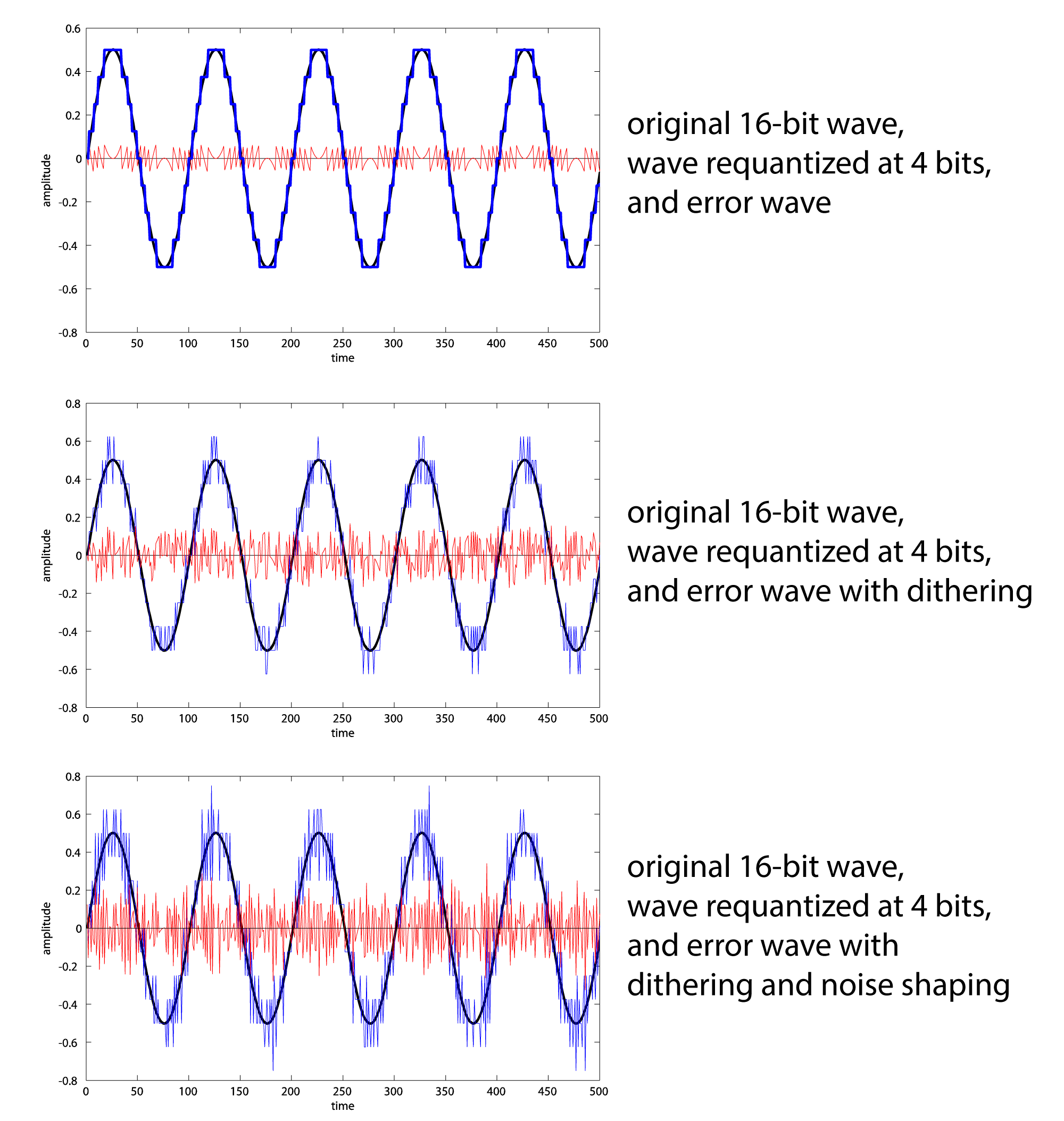
Requantization without dithering, with dithering, and with dithering and noise shaping are compared in Figure 5.41.   A 16-bit audio file has been requantized to 4 bits (an unlikely scenario, but it makes the point).   From these graphs, it may look like noise shaping adds additional noise. In fact, the reason the noise graph looks more dense when noise shaping is added is that the frequency components are higher.

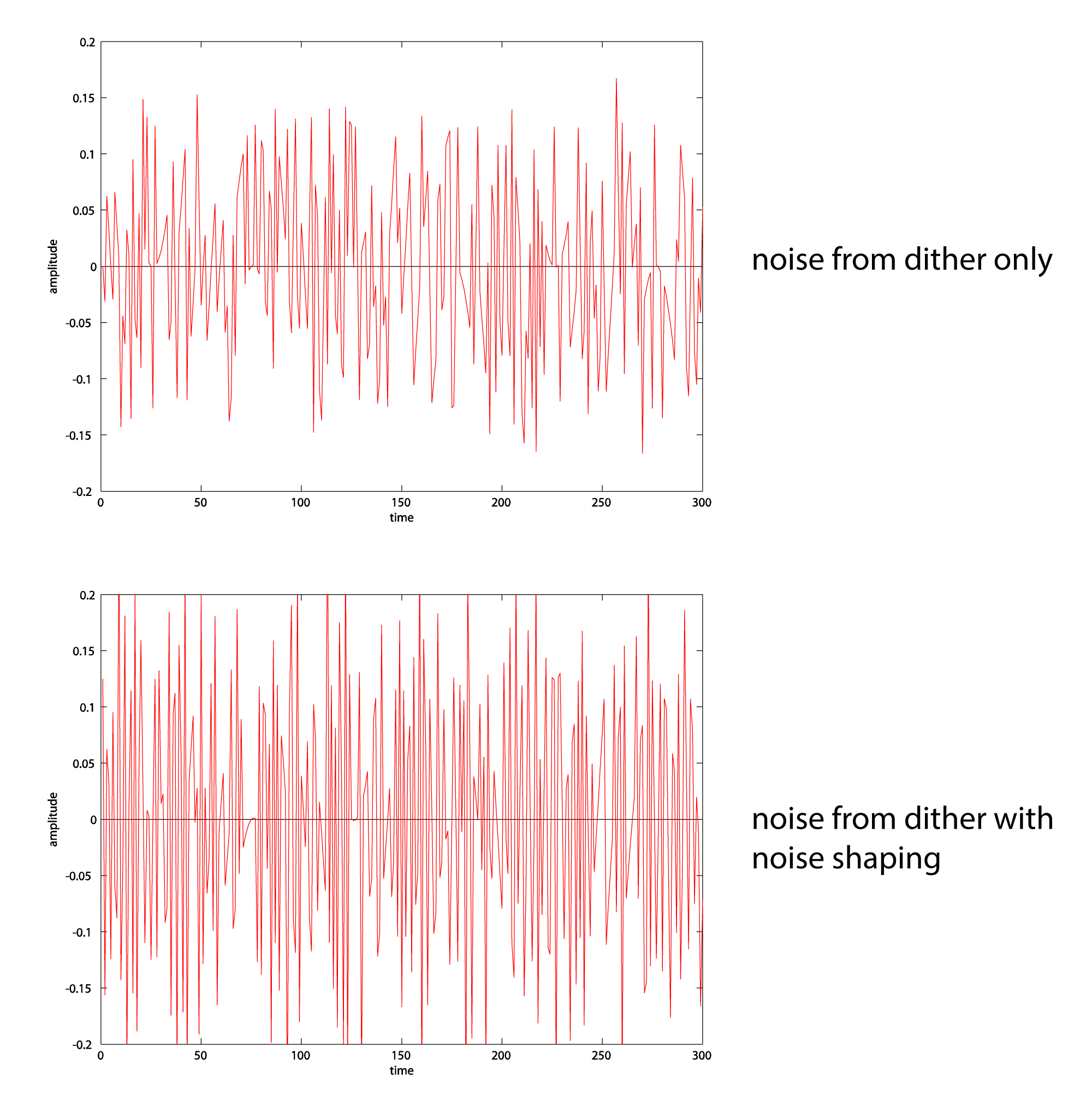
To examine this more closely, we can extract the noise into a separate audio file by subtracting the original file from the requantized one. We’ve done this for both cases – noise from dither, and noise from dither and noise shaping. (The noise includes the quantization error.) Closeups of the noise graphs are shown in Figure 5.42. What you should notice is that dither-with-noise-shaping noise has higher frequency components than dither-only noise.

You can see this also in the spectral view of the noise files in Figure 5.43. In a spectral view of an audio file, time is on the x-axis, frequency is on the y-axis, and the amplitude of the frequency is represented by the color at each (x,y) point. The lowest amplitude is represented by blue, medium amplitudes move from red to orange, and the highest amplitudes move from yellow to white. You can see that when dithering alone is applied, the noise is spread out over all frequencies. When noise shaping is added to dithering, there is less noise at low frequency and more noise at high frequency. The effect is to pull more of the noise to high frequencies, where it is noticed less by human ears. (ADCs also can filter out the high frequency noise if it is above the Nyquist frequency.)

Noise shaping algorithms, first developed by Cutler in the 1950s, operate by computing the error from quantizing a sample (including the error from dithering and noise shaping) and adding this error to the next sample before it is quantized. If the error from the i^th sample is positive, then, by subtracting the error from the next sample, noise shaping makes it more likely that the error for the i+1^st sample will be negative. This causes the error wave to go up and down more frequently; i.e., the frequency of the error wave is increased. The algorithm is given in Algorithm 5.2. You can output your files as uncompressed RAW files, import the data into MATLAB, and graph the error waves, comparing the shape of the error with dither-only and with noise shaping using various values for c, the scaling factor. The algorithm given is the most basic kind of noise shaping you can do. Many refinements and variations of this algorithm have been implemented and distributed commercially.

[equation class=”algorithm” caption=”Algorithm 5.2″]

algorithm noise_shape {
/*Input:
     b_orig, the original bit depth
     b_new, the new bit depth to which samples are to be quantized
     F_in, an array of N digital audio samples that are to be
     quantized, dithered, and noise shaped.  It’s assumed that these are read
     in from a RAW file and are values between
     –2^b_orig-1 and (2^b_orig-1)-1.
     c, a scaling factor for the noise shaping
Output:
     F_out, an array of N digital audio samples quantized to bit
     depth b_new using dither and noise shaping*/

   s = (2^b_orig)/(2^b_new);
   c = 0.8;  //Other scaling factors can be tried.*/
   e = 0;
   for (i = 0; i < N; i++) {
/*Get a random number between −1 and 1 from some probability density function*/
      d = pdf();
      F_scaled  = F_in[i] / s;  //Integer division, discarding remainder
      F_scaled_plus_dith_and_error = F_scaled + d + c*e;
      F_out[i] =  floor(F_scaled_plus_dith_and_error);
      e = F_scaled – F_out[i];
   }
}

[/equation]