Many of the concepts introduced in Sections 5.1 and 5.2 may become clearer if you experiment with the mathematics, visualize or listen to the audio data in MATLAB, or write some of the algorithms to see the results first-hand. We’ll try that in this section.
It’s possible to predict the frequency of an aliased wave in cases where aliasing occurs. The algorithm for this is given in Algorithm 5.1. There are four cases to consider. We’ll use a sampling rate of 1000 Hz to illustrate the algorithm. At this sampling rate, the Nyquist frequency is 500 Hz.
[equation class=”algorithm” caption=”Algorithm 5.1″]
algorithm aliasing {
/*Input:
Frequency of a single-frequency sound wave to be sampled, f_act
     Sampling rate, f_samp
Output:
     Frequency of the digitized audio wave, f_obs*/
   f_nf = 1/2 * f_samp   //Nyquist frequency is 1/2 sampling rate
   if (f_act <= f_nf)                 //Case 1, no aliasing
      f_obs = f_act
   else if (f_nf < f_act <= f_samp)   //Case 2
      f_obs = f_samp – f_act;
   else {
      p = f_act / f_nf   //integer division, drop remainder
      r = f_act mod f_nf	//remainder from integer division
	   if (p is even) then           //Case 3
         f_obs = r;
      else if (p is odd) then         //Case 4
         f_obs = f_nf – r;
   }
}
[/equation]
[wpfilebase tag=file id=123 tpl=supplement /]
In the first case, when the actual frequency is less than or equal to the Nyquist frequency, the sampling rate is sufficient and there is no aliasing. In the second case, when the actual frequency is between the Nyquist frequency and the sampling rate, the observed frequency is equal to the sampling rate minus the actual frequency. For example, a sampling rate of 1000 Hz causes an 880 Hz sound wave to alias to 120 Hz (Figure 5.35).
For an actual frequency that is above the sampling rate, like 1320 Hz, the calculations are as follows:
$$p=1320/500=2$$
$$r=1320\,mod\,500=320$$
p is even, so
$$f_{obs}=320$$
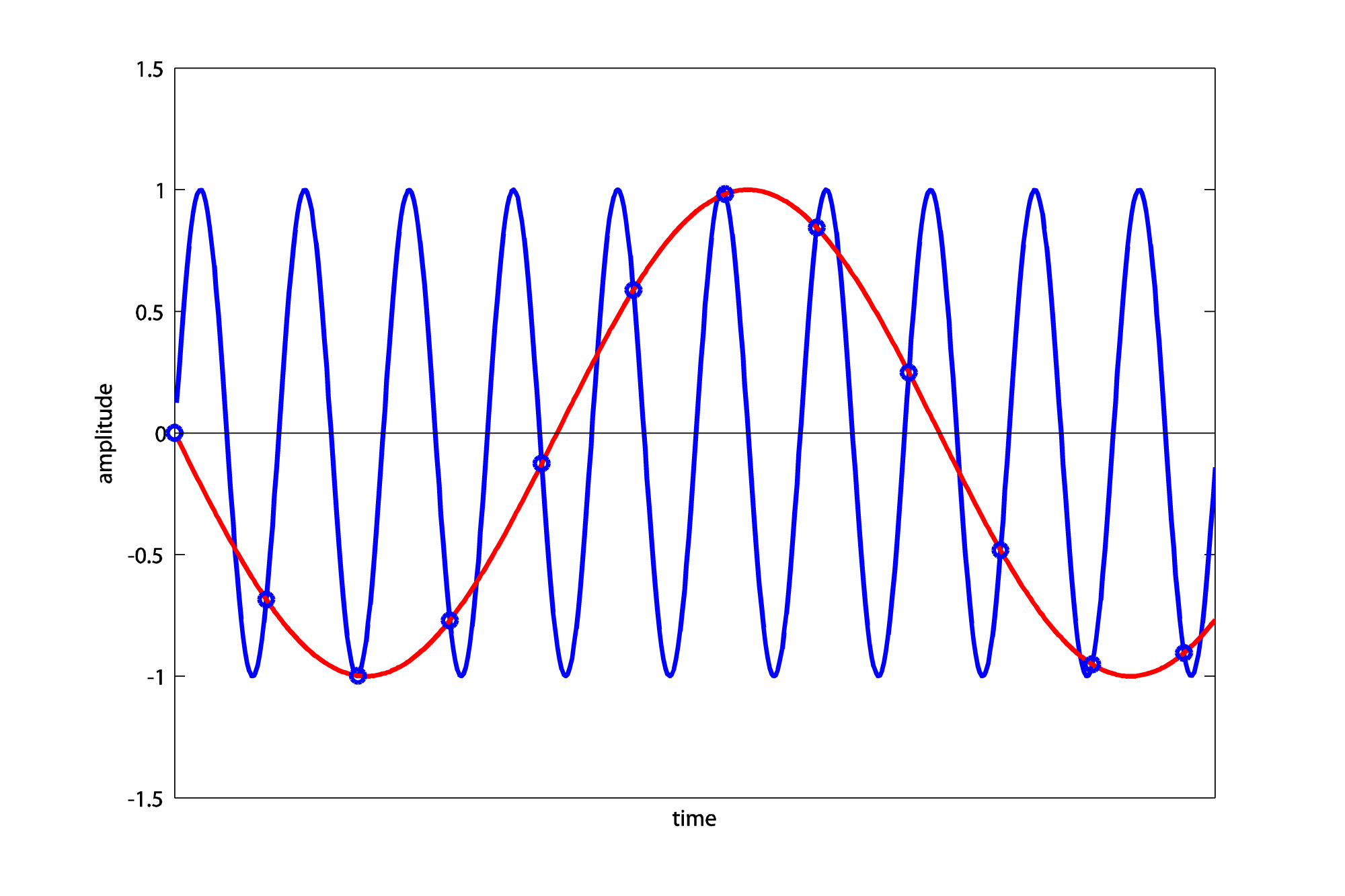
Thus, a 1320 Hz wave sampled at 1000 Hz aliases to 320 Hz (Figure 5.36).
For an actual frequency of 1760 Hz, we have
$$p=1760/500=3$$
$$r=1760\,mod\,500=260$$
p is odd, so
$$f_{obs}=500-260=240$$
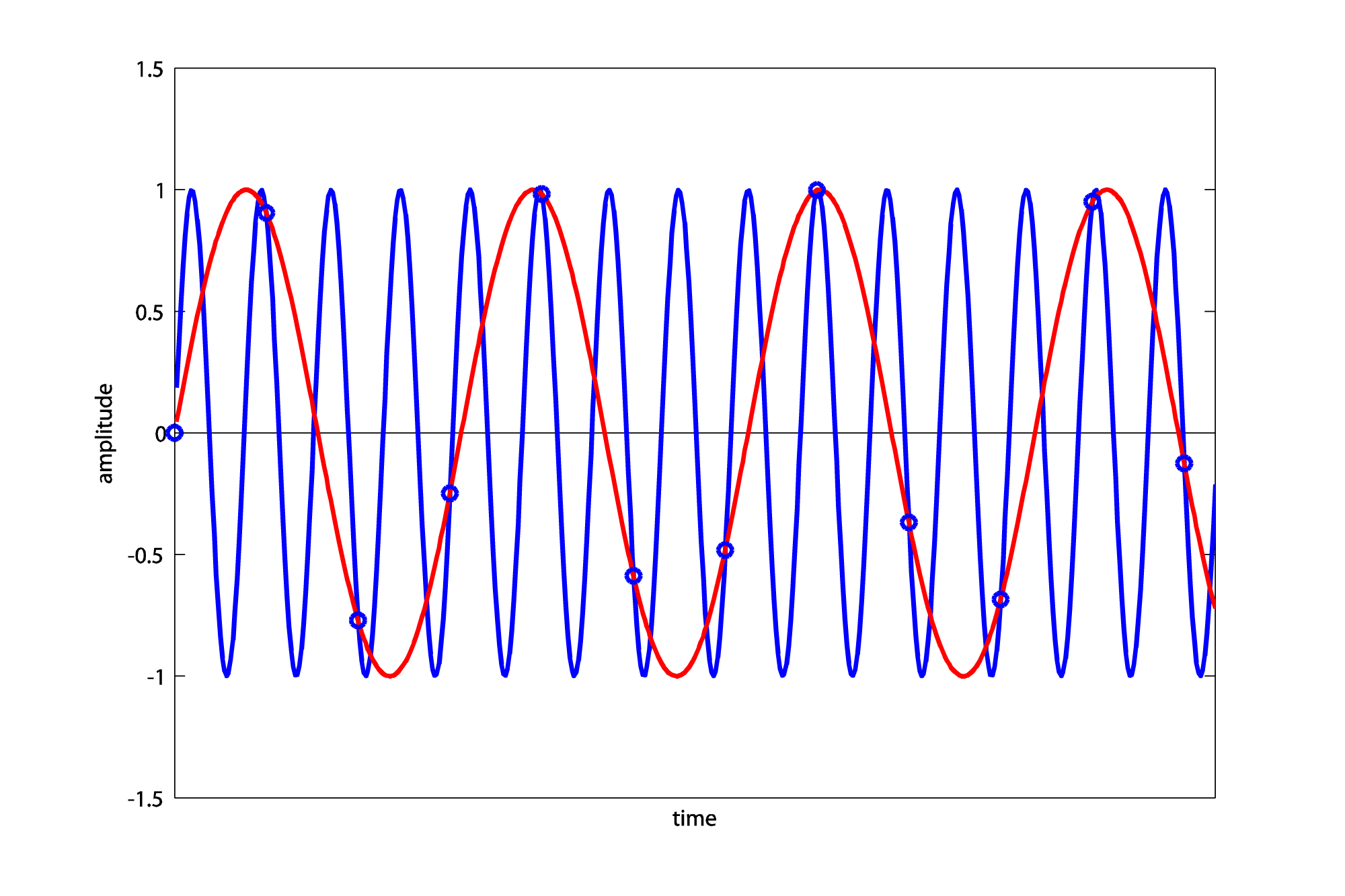
Thus, a 1760 Hz wave sampled at 1000 Hz aliases to 240 Hz (Figure 5.37).

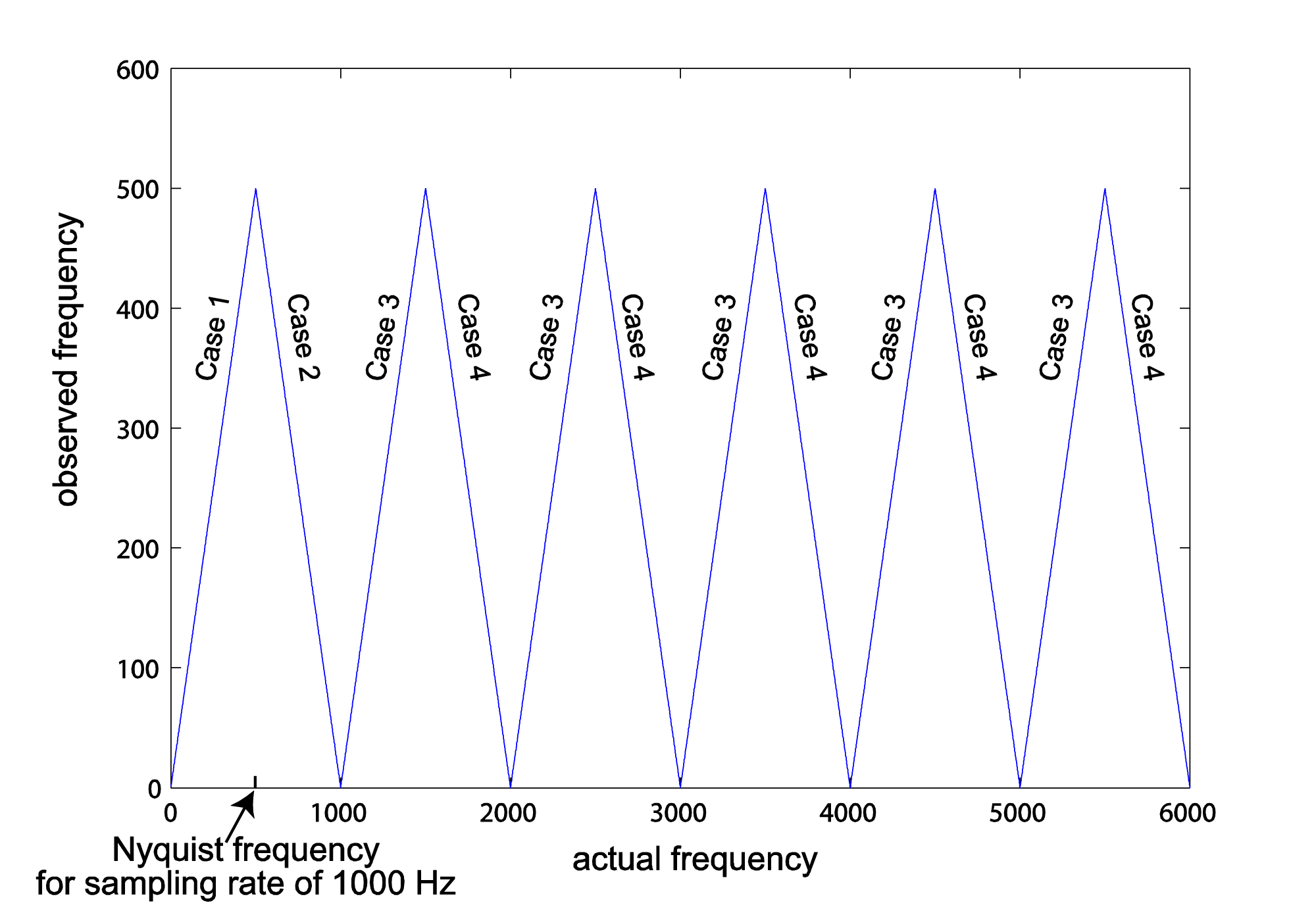
The graph in Figure 5.38 shows f_obs as a function of f_act for a fixed sampling rate, in this case 1000 Hz. For a different sampling rate, the graph would still have the same basic repeated-peak shape, but its peaks would be at different places. The first peak from the left is located at the Nyquist frequency on the horizontal axis, which is half the sampling rate. After the first peak, Case 3 is always on the left side of a peak and Case 4 is always on the right.