4.1.5.1 Why Decibels for Sound?
No doubt you’re familiar with the use of decibels related to sound, but let’s look more closely at the definition of decibels and why they are a good way to represent sound levels as they’re perceived by human ears.
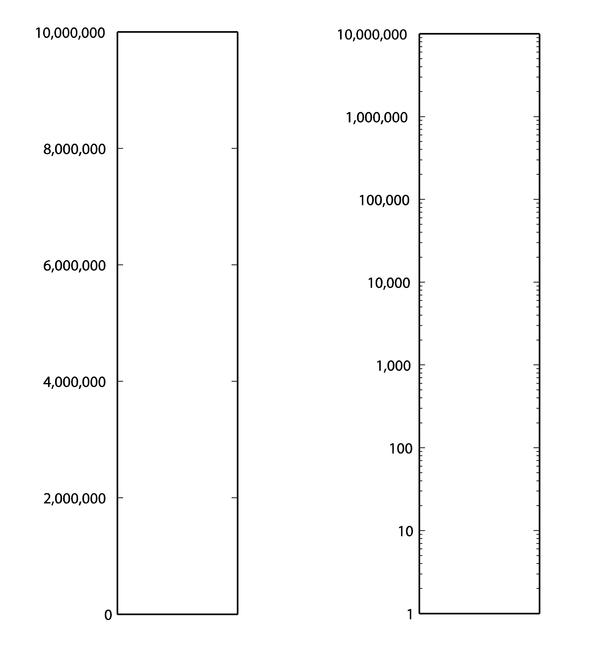
First consider Table 4.1. From column 3, you can see that the sound of a nearby jet engine has on the order of times greater air pressure amplitude than the threshold of hearing. That’s quite a wide range. Imagine a graph of sound loudness that has perceived loudness on the horizontal axis and air pressure amplitude on the vertical axis. We would need numbers ranging from 0 to 10,000,000 on the vertical axis (Figure 4.1). This axis would have to be compressed to fit on a sheet of paper or a computer screen, and we wouldn’t see much space between, say, 100 and 200. Thus, our ability to show small changes at low amplitude would not be great. Although we perceive a vacuum cleaner to be approximately twice as loud as normal conversation, we would hardly be able to see any difference between their respective air pressure amplitudes if we have to include such a wide range of numbers, spacing them evenly on what is called a linear scale. A linear scale turns out to be a very poor representation of human hearing. We humans can more easily distinguish the difference between two low amplitude sounds that are close in amplitude than we can distinguish between two high amplitude sounds that are close in amplitude. The linear scale for loudness doesn’t provide sufficient resolution at low amplitudes to show changes that might actually be perceptible to the human ear.
[table caption=”Table 4.1 Loudness of common sounds measured in air pressure amplitude and in decibels” width=”80%”]
Sound,Approximate Air Pressure~~Amplitude in Pascals,Ratio of Sound’s Air Pressure~~Amplitude to Air Pressure Amplitude~~of Threshold of Hearing,Approximate Loudness~~in dBSPL
Threshold of hearing,$$0.00002 = 2 \ast 10^{-5}$$ ,1,0
Breathing,$$0.00006325 = 6.325 \ast 10^{-5}$$ ,3.16,10
Rustling leaves,$$0.0002=2\ast 10^{-4}$$,10,20
Refrigerator humming,$$0.002 = 2 \ast 10^{-3}$$ ,$$10^{2}$$,40
Normal conversation,$$0.02 = 2\ast 10^{-2}$$ ,$$10^{3}$$,60
Vacuum cleaner,$$0.06325 =6.325 \ast 10^{-2}$$ ,$$3.16 \ast 10^{3}$$,70
Dishwasher,$$0.1125 = 1.125 \ast 10^{-1}$$,$$5.63 \ast 10^{3}$$,75
City traffic,$$0.2 = 2 \ast 10^{-1}$$,$$10^{4}$$,80
Lawnmower,$$0.3557 = 3.557 \ast 10^{-1}$$,$$1.78 \ast 10^{4}$$,85
Subway,$$0.6325 = 6.325 \ast 10^{-1}$$,$$3.16 \ast 10^{4}$$,90
Symphony orchestra,6.325,$$3.16 \ast 10^{5}$$,110
Fireworks,$$20 = 2 \ast 10^{1}$$,$$10^{6}$$,120
Rock concert,$$20+ = 2 \ast 10^{1}+$$,$$10^{6}+$$,120+
Shotgun firing,$$63.25 = 6.325 \ast 10^{1}$$,$$3.16 \ast 10^{6}$$,130
Jet engine close by,$$200 = 2 \ast 10^{2}$$,$$2 \ast 10^{7}$$,140
[/table]
Now let’s see how these observations begin to help us make sense of the decibel. A decibel is based on a ratio – that is, one value relative to another, as in $$\frac{X_{1}}{X_{0}}$$. Hypothetically, $$X_{0}$$ and $$X_{1}$$ could measure anything, as long as they measure the same type of thing in the same units – e.g., power, intensity, air pressure amplitude, noise on a computer network, loudspeaker efficiency, signal-to-noise ratio, etc. Because decibels are based on a ratio, they imply a comparison. Decibels can be a measure of
- a change from level $$X_{0}$$ to level $$X_{1}$$
- a range of values between $$X_{0}$$ and $$X_{1}$$, or
- a level $$X_{1}$$ compared to some agreed upon reference point $$X_{0}$$.
What we’re most interested in with regard to sound is some way of indicating how loud it seems to human ears. What if we were to measure relative loudness using the threshold of hearing as our point of comparison – the $$X_{0}$$, in the ratio $$\frac{X_{1}}{X_{0}}$$, as in column 3 of Table 4.1? That seems to make sense. But we already noted that the ratio of the loudest to the softest thing in our table is 10,000,000/1. A ratio alone isn’t enough to turn the range of human hearing into manageable numbers, nor does it account for the non-linearity of our perception.
The discussion above is given to explain why it makes sense to use the logarithm of the ratio of $$\frac{X_{1}}{X_{0}}$$ to express the loudness of sounds, as shown in Equation 4.4. Using the logarithm of the ratio, we don’t have to use such widely-ranging numbers to represent sound amplitudes, and we “stretch out” the distance between the values corresponding to low amplitude sounds, providing better resolution in this area.
The values in column 4 of Table 4.1, measuring sound loudness in decibels, come from the following equation for decibels-sound-pressure-level, abbreviated dBSPL.
[equation caption=”Equation 4.4 Definition of dBSPL, also called ΔVoltage”]
$$!dBSPL = \Delta Voltage \; dB=20\log_{10}\left ( \frac{V_{1}}{V_{0}} \right )$$
[/equation]
In this definition, $$V_{0}$$ is the air pressure amplitude at the threshold of hearing, and $$V_{1}$$ is the air pressure amplitude of the sound being measured.
Notice that in Equation 4.4, we use ΔVoltage dB as synonymous with dBSPL. This is because microphones measure sound as air pressure amplitudes, turn the measurements into voltages levels, and convey the voltage values to an audio interface for digitization. Thus, voltages are just another way of capturing air pressure amplitude.
Notice also that because the dimensions are the same in the numerator and denominator of $$\frac{V_{1}}{V_{0}}$$, the dimensions cancel in the ratio. This is always true for decibels. Because they are derived from a ratio, decibels are dimensionless units. Decibels aren’t volts or watts or pascals or newtons; they’re just the logarithm of a ratio.
Hypothetically, the decibel can be used to measure anything, but it’s most appropriate for physical phenomena that have a wide range of levels where the values grow exponentially relative to our perception of them. Power, intensity, and air pressure amplitude are three physical phenomena related to sound that can be measured with decibels. The important thing in any usage of the term decibels is that you know the reference point – the level that is in the denominator of the ratio. Different usages of the term decibel sometimes add different letters to the dB abbreviation to clarify the context, as in dBPWL (decibels-power-level), dBSIL (decibels-sound-intensity-level), and dBFS (decibels-full-scale), all of which are explained below.
Comparing the columns in Table 4.1, we now can see the advantages of decibels over air pressure amplitudes. If we had to graph loudness using Pa as our units, the scale would be so large that the first ten sound levels (from silence all the way up to subways) would not be distinguishable from 0 on the graph. With decibels, loudness levels that are easily distinguishable by the ear can be seen as such on the decibel scale.
Decibels are also more intuitively understandable than air pressure amplitudes as a way of talking about loudness changes. As you work with sound amplitudes measured in decibels, you’ll become familiar with some easy-to-remember relationships summarized in Table 4.2. In an acoustically-insulated lab environment with virtually no background noise, a 1 dB change yields the smallest perceptible difference in loudness. However, in average real-world listening conditions, most people can’t notice a loudness change less than 3 dB. A 10 dB change results in about a doubling of perceived loudness. It doesn’t matter if you’re going from 60 to 70 dBSPL or from 80 to 90 dBSPL. The increase still sounds approximately like a doubling of loudness. In contrast, going from 60 to 70 dBSPL is an increase of 43.24 mPa, while going from 80 to 90 dBSPL is an increase of 432.5 mPa. Here you can see that saying that you “turned up the volume” by a certain air pressure amplitude wouldn’t give much information about how much louder it’s going to sound. Talking about loudness-changes in terms of decibels communicates more.
[table caption=”Table 4.2 How sound level changes in dB are perceived”]
Change of sound amplitude,How it is perceived in human hearing
1 dB,”smallest perceptible difference in loudness, only perceptible in acoustically-insulated noiseless environments”
3 dB,smallest perceptible change in loudness for most people in real-world environments
+10 dB,an approximate doubling of loudness
-10 dB change,an approximate halving of loudness
[/table]
You may have noticed that when we talk about a “decibel change,” we refer to it as simply decibels or dB, whereas if we are referring to a sound loudness level relative to the threshold of hearing, we refer to it as dBSPL. This is correct usage. The difference between 90 and 80 dBSPL is 10 dB. The difference between any two decibels levels that have the same reference point is always measured in dimensionless dB. We’ll return to this in a moment when we try some practice problems in Section 2.
4.1.5.2 Various Usages of Decibels
Now let’s look at the origin of the definition of decibel and how the word can be used in a variety of contexts.
The bel, named for Alexander Graham Bell, was originally defined as a unit for measuring power. For clarity, we’ll call this the power difference bel, also denoted :
[equation caption=”Equation 4.5 , power difference bel”]
$$!1\: power\: difference\: bel=\Delta Power\: B=\log_{10}\left ( \frac{P_{1}}{P_{0}} \right )$$
[/equation]
The decibel is 1/10 of a bel. The decibel turns out to be a more useful unit than the bel because it provides better resolution. A bel doesn’t break measurements into small enough units for most purposes.
We can derive the power difference decibel (Δ Power dB) from the power difference bel simply by multiplying the log by 10. Another name for ΔPower dB is dBPWL (decibels-power-level).
[equation caption=”Equation 4.6, abbreviated dBPWL”]
$$!\Delta Power\: B=dBPWL=10\log_{10}\left ( \frac{P_{1}}{P_{0}} \right )$$
[/equation]
When this definition is applied to give a sense of the acoustic power of a sound, then is the power of sound at the threshold of hearing, which is $$10^{-12}W=1pW$$ (picowatt).
Sound can also be measured in terms of intensity. Since intensity is defined as power per unit area, the units in the numerator and denominator of the decibel ratio are $$\frac{W}{m^{2}}$$, and the threshold of hearing intensity is $$10^{-12}\frac{W}{m^{2}}$$. This gives us the following definition of ΔIntensity dB, also commonly referred to as dBSIL (decibels-sound intensity level).
[equation caption=”Equation 4.7 , abbreviated dBSIL”]
$$!\Delta Intensity\, dB=dBSIL=10\log_{10}\left ( \frac{I_{1}}{I_{0}} \right )$$
[/equation]
Neither power nor intensity is a convenient way of measuring the loudness of sound. We give the definitions above primarily because they help to show how the definition of dBSPL was derived historically. The easiest way to measure sound loudness is by means of air pressure amplitude. When sound is transmitted, air pressure changes are detected by a microphone and converted to voltages. If we consider the relationship between voltage and power, we can see how the definition of ΔVoltage dB was derived from the definition of ΔPower dB. By Equation 4.3, we know that power varies with the square of voltage. From this we get: $$!10\log_{10}\left ( \frac{P_{1}}{P_{0}} \right )=10\log_{10}\left ( \left ( \frac{V_{1}}{V_{0}} \right )^{2} \right )=20\log_{10}\left ( \frac{V_{1}}{V_{0}} \right )$$ The relationship between power and voltage explains why there is a factor of 20 is in Equation 4.4.
[aside width=”125px”]
$$\log_{b}\left ( y^{x} \right )=x\log_{b}y$$
[/aside]
We can show how Equation 4.4 is applied to convert from air pressure amplitude to dBSPL and vice versa. Let’s say we begin with the air pressure amplitude of a humming refrigerator, which is about 0.002 Pa.
$$!dBSPL=20\log_{10}\left ( \frac{0.002\: Pa}{0.00002\: Pa} \right )=20\log_{10}\left ( 100 \right )=20\ast 2=40\: dBSPL$$
Working in the opposite direction, you can convert the decibel level of normal conversation (60 dBSPL) to air pressure amplitude:
$$\begin{align*}& 60=20\log_{10}\left ( \frac{0.002\: Pa}{0.00002\: Pa} \right )=20\log_{10}\left ( 50000x/Pa \right ) \\&\frac{60}{20}=\log_{10}\left ( 50000x/Pa \right ) \\&3=\log_{10}\left ( 50000x/Pa \right ) \\ &10^{3}= 50000x/Pa\\&x=\frac{1000}{50000}Pa \\ &x=0.02\: Pa \end{align*}$$
[aside width=”125px”]
If $$x=\log_{b}y$$
then $$b^{x}=y$$
[/aside]
Thus, 60 dBSPL corresponds to air pressure amplitude of 0.02 Pa.
Rarely would you be called upon to do these conversions yourself. You’ll almost always work with sound intensity as decibels. But now you know the mathematics on which the dBSPL definition is based.
So when would you use these different applications of decibels? Most commonly you use dBSPL to indicate how loud things seem relative to the threshold of hearing. In fact, you use this type of decibel so commonly that the SPL is often dropped off and simply dB is used where the context is clear. You learn that human speech is about 60 dB, rock music is about 110 dB, and the loudest thing you can listen to without hearing damage is about 120 dB – all of these measurements implicitly being dBSPL.
The definition of intensity decibels, dBSIL, is mostly of interest to help us understand how the definition of dBSPL can be derived from dBPWL. We’ll also use the definition of intensity decibels in an explanation of the inverse square law, a rule of thumb that helps us predict how sound loudness decreases as sound travels through space in a free field (Section 4.2.1.6).
There’s another commonly-used type of decibel that you’ll encounter in digital audio software environments – the decibel-full-scale (dBFS). You may not understand this type of decibel completely until you’ve read Chapter 5 because it’s based on how audio signals are digitized at a certain bit depth (the number of bits used for each audio sample). We’ll give the definition here for completeness and revisit it in Chapter 5. The definition of dBFS uses the largest-magnitude sample size for a given bit depth as its reference point. For a bit depth of n, this largest magnitude would be $$2^{n-1}$$.
[equation caption=”Equation 4.8 Decibels-full-scale, abbreviated dBFS”]
$$!dBFS = 20\log_{10}\left ( \frac{\left | x \right |}{2^{n-1}} \right )$$
where n is a given bit depth and x is an integer sample value between $$-2^{n-1}$$ and $$2^{n-1}-1$$.
[/equation]
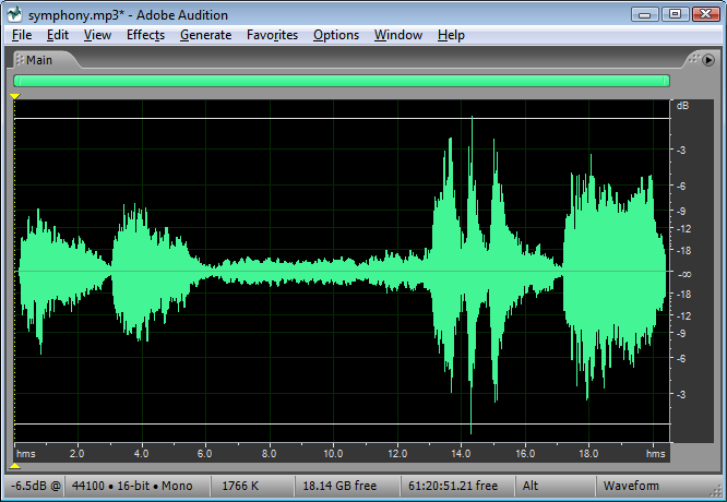
Figure 4.2 shows an audio processing environment where a sound wave is measured in dBFS. Notice that since $$\left | x \right |$$ is never more than $$2^{n-1}$$, $$log_{10}\left ( \frac{\left | x \right |}{2^{n-1}} \right )$$ is never a positive number. When you first use dBFS it may seem strange because all sound levels are at most 0. With dBFS, 0 represents maximum amplitude for the system, and values move toward -∞ as you move toward the horizontal axis, i.e., toward quieter sounds.
The discussion above has considered decibels primarily as they measure sound loudness. Decibels can also be used to measure relative electrical power or voltage. For example, dBV measures voltage using 1 V as a reference level, dBu measures voltage using 0.775 V as a reference level, and dBm measures power using 0.001 W as a reference level. These applications come into play when you’re considering loudspeaker or amplifier power, or wireless transmission signals. In Section 2, we’ll give you some practical applications and problems where these different types of decibels come into play.
The reference levels for different types of decibels are listed in Table 4.3. Notice that decibels are used in reference to the power of loudspeakers or the input voltage to audio devices. We’ll look at these applications more closely in Section 2. Of course, there are many other common usages of decibels outside of the realm of sound.
[table caption=”Table 4.3 Usages of the term decibels with different reference points” width=”80%”]
what is being measured,abbreviations in common usage,common reference point,equation for conversion to decibels
Acoustical,,,
sound power ,dBPWL or ΔPower dB,$$P_{0}=10^{-12}W=1pW(picowatt)$$ ,$$10\log_{10}\left ( \frac{P_{1}}{P_{0}} \right )$$
sound intensity ,dBSIL or ΔIntensity dB,”threshold of hearing, $$I_{0}=10^{-12}\frac{W}{m^{2}}”$$,$$10\log_{10}\left ( \frac{I_{1}}{i_{0}} \right )$$
sound air pressure amplitude ,dBSPL or ΔVoltage dB,”threshold of hearing, $$P_{0}=0.00002\frac{N}{m^{2}}=2\ast 10^{-5}Pa$$”, $$20\log_{10}\left ( \frac{V_{1}}{V_{0}} \right )$$
sound amplitude,dBFS, “$$2^{n-1}$$ where n is a given bit depth x is a sample value, $$-2^{n-1} \leq x \leq 2^{n-1}-1$$”,dBFS=$$20\log_{10}\left ( \frac{\left | x \right |}{2^{n-1}} \right )$$
Electrical,,,
radio frequency transmission power,dBm,$$P_{0}=1 mW = 10^{-3} W$$ ,$$10\log_{10}\left ( \frac{P_{1}}{P_{0}} \right )$$
loudspeaker acoustical power,dBW,$$P_{0}=1 W$$,$$10\log_{10}\left ( \frac{P_{1}}{P_{0}} \right )$$
input voltage from microphone; loudspeaker voltage; consumer level audio voltage,dBV,$$V_{0}=1 V$$,$$20\log_{10}\left ( \frac{V_{1}}{V_{0}} \right )$$
professional level audio voltage,dBu,$$V_{0}=0.775 V$$,$$20\log_{10}\left ( \frac{V_{1}}{V_{0}} \right )$$
[/table]
4.1.5.3 Peak Amplitude vs. RMS Amplitude
Microphones and sound level meters measure the amplitude of sound waves over time. There are situations in which you may want to know the largest amplitude over a time period. This “largest” can be measured in one of two ways: as peak amplitude or as RMS amplitude.
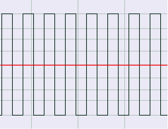
Let’s assume that the microphone or sound level meter is measuring sound amplitude. The sound pressure level of greatest magnitude over a given time period is called the peak amplitude. For a single-frequency sound representable by a sine wave, this would be the level at the peak of the sine wave. The sound represented by Figure 4.3 would obviously be perceived as louder than the same-frequency sound represented by Figure 4.4. However, how would the loudness of a sine-wave-shaped sound compare to the loudness of a square-wave-shaped sound with the same peak amplitude (Figure 4.3 vs. Figure 4.5)? The square wave would actually sound louder. This is because the square wave is at its peak level more of the time as compared to the sine wave. To account for this difference in perceived loudness, RMS amplitude (root-mean-square amplitude) can be used as an alternative to peak amplitude, providing a better match for the way we perceive the loudness of the sound.


Rather than being an instantaneous peak level, RMS amplitude is similar to a standard deviation, a kind of average of the deviation from 0 over time. RMS amplitude is defined as follows:
[equation caption=”Equation 4.9 Equation for RMS amplitude, $$V_{RMS}$$”]
$$!V_{RMS}=\sqrt{\frac{\sum _{i=1}^{n}\left ( S_{i} \right )^{2}}{n}}$$
where n is the number of samples taken and $$S_{i}$$ is the $$i^{th}$$ sample.
[/equation]
[aside]In some sources, the term RMS power is used interchangeably with RMS amplitude or RMS voltage. This isn’t very good usage. To be consistent with the definition of power, RMS power ought to mean “RMS voltage multiplied by RMS current.” Nevertheless, you sometimes see term RMS power used as a synonym of RMS amplitude as defined in Equation 4.9.[/aside]
Notice that squaring each sample makes all the values in the summation positive. If this were not the case, the summation would be 0 (assuming an equal number of positive and negative crests) since the sine wave is perfectly symmetrical.
The definition in Equation 4.9 could be applied using whatever units are appropriate for the context. If the samples are being measured as voltages, then RMS amplitude is also called RMS voltage. The samples could also be quantized as values in the range determined by the bit depth, or the samples could also be measured in dimensionless decibels, as shown for Adobe Audition in Figure 4.6.
For a pure sine wave, there is a simple relationship between RMS amplitude and peak amplitude.
[equation caption=”Equation 4.10 Relationship between $$V_{rms}$$ and $$V_{peak}$$ for pure sine waves”]
for pure sine waves
$$!V_{RMS}=\frac{V_{peak}}{\sqrt{2}}=0.707\ast V_{peak}$$
and
$$!V_{peak}=1.414\ast V_{RMS}$$
[/equation]
Of course most of the sounds we hear are not simple waveforms like those shown; natural and musical sounds contain many frequency components that vary over time. In any case, the RMS amplitude is a better model for our perception of the loudness of complex sounds than is peak amplitude.
Sound processing programs often give amplitude statistics as either peak or RMS amplitude or both. Notice that RMS amplitude has to be defined over a particular window of samples, labeled as Window Width in Figure 4.6. This is because the sound wave changes over time. In the figure, the window width is 1000 ms.

You need to be careful will some usages of the term “peak amplitude.” For example, VU meters, which measure signal levels in audio equipment, use the word “peak” in their displays, where RMS amplitude would be more accurate. Knowing this is important when you’re setting levels for a live performance, as the actual peak amplitude is higher than RMS. Transients like sudden percussive noises should be kept well below what is marked as “peak” on a VU meter. If you allow the level to go too high, the signal will be clipped.