Generally when you work with digital audio, you don’t have to implement your own FFT. Efficient implementations already exist in many programming language libraries. For example, MATLAB has FFT and inverse FFT functions, fft and ifft, respectively. We can use these to experiment and generate graphs of sound data in the frequency domain. First, let’s use sine functions to generate arrays of numbers that simulate single-pitch sounds. We’ll make three one-second long sounds using the standard sampling rate for CD quality audio, 44,100 samples per second. First, we generate an array of sr*s numbers across which we can evaluate sine functions, putting this array in the variable t.
sr = 44100; %sr is sampling rate
s = 1; %s is number of seconds
t = linspace(0, s, sr*s);
Now we use the array t as input to sine functions at three different frequencies and phases, creating the note A at three different octaves (110 Hz, 220 Hz, and 440 Hz).
x = cos(2*pi*110*t);
y = cos(2*pi*220*t + pi/3);
z = cos(2*pi*440*t + pi/6);
x, y, and z are arrays of numbers that can be used as audio samples. pi/3 and pi/6 represent phase shifts for the 220 Hz and 440 Hz waves, to make our phase response graph more interesting. The figures can be displayed with the following:
figure;
plot(t,x);
axis([0 0.05 -1.5 1.5]);
title('x');
figure;
plot(t,y);
axis([0 0.05 -1.5 1.5]);
title('y');
figure;
plot(t,z);
axis([0 0.05 -1.5 1.5]);
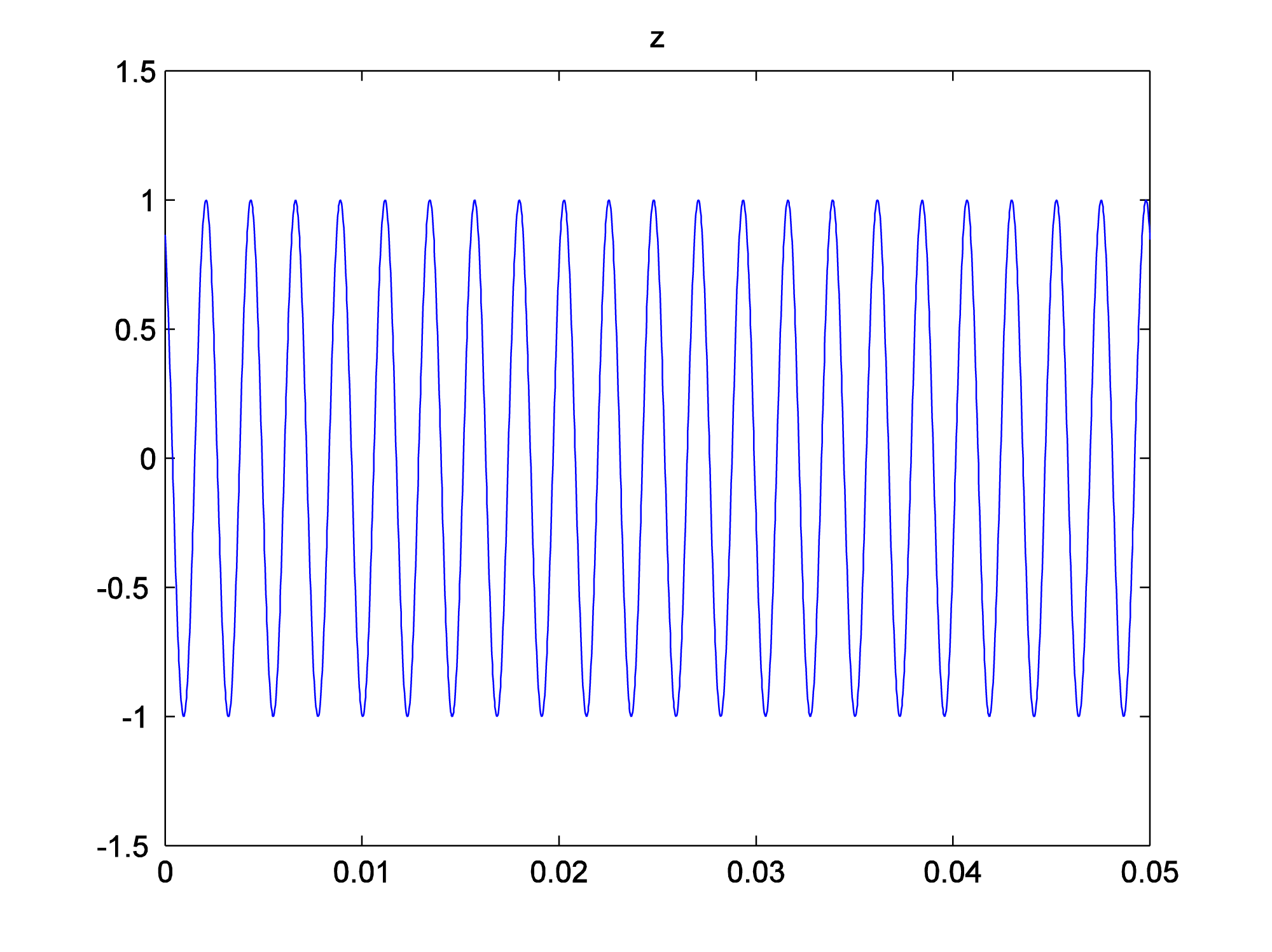
title('z');
We look at only the first 0.05 seconds of the waveforms in order to see their shape better. You can see the phase shifts in the figures below. The second and third waves don’t start at 0 on the vertical axis.


Now we add the three sine waves to create a composite wave that has three frequency components at three different phases.
a = (x + y + z)/3;
Notice that we divide the summed sound waves by three so that the sound doesn’t clip. You can graph the three-component sound wave with the following:
figure;
plot(t, a);
axis([0 0.05 -1.5 1.5]);
title('a = x + y + z');
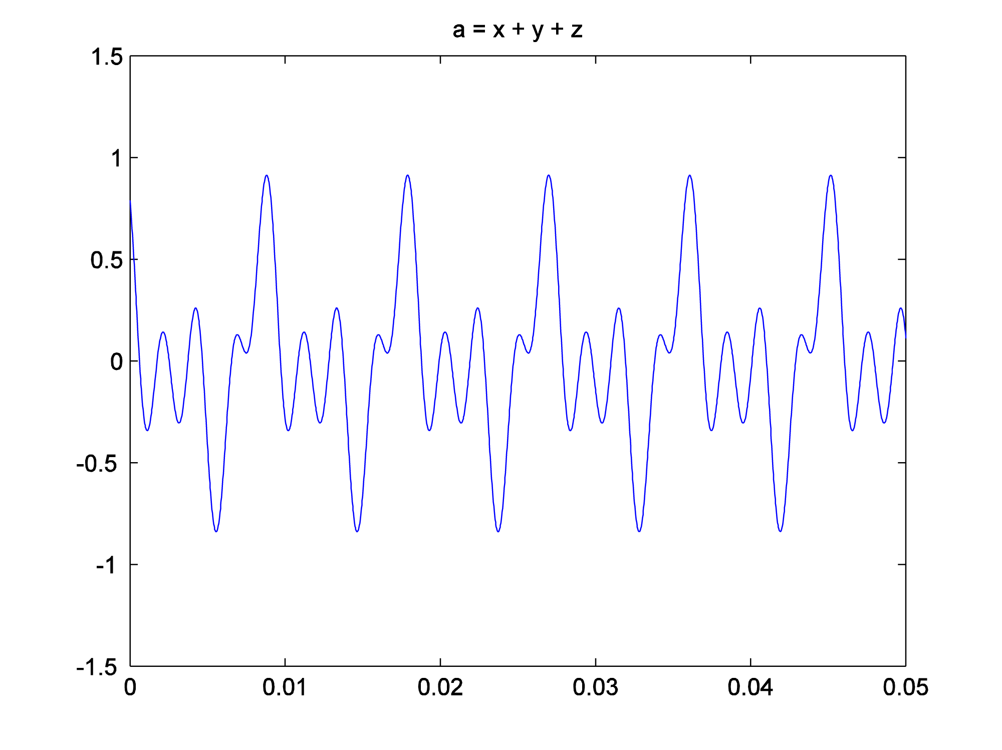
This is a graph of the sound wave in the time domain. You could call it an impulse response graph, although when you’re looking at a sound file like this, you usually just think of it as “sound data in the time domain.” The term “impulse response” is used more commonly for time domain filters, as we’ll see in Chapter 7. You might want to play the sound to be sure you have what you think you have. The sound function requires that you tell it the number of samples it should play per second, which for our simulation is 44,100.
sound(a, sr);
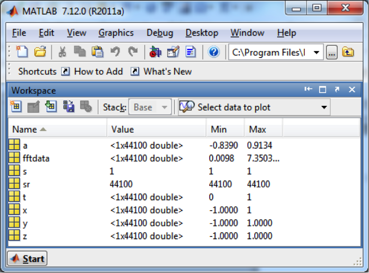
When you play the sound file and listen carefully, you can hear that it has three tones. MATLAB’s Fourier transform (fft) returns an array of double complex values (double-precision complex numbers) that represent the magnitudes and phases of the frequency components.
fftdata = fft(a);
In MATLAB’s workspace window, fftdata values are labeled as type double, giving the impression that they are real numbers, but this is not the case. In fact, the Fourier transform produces complex numbers, which you can verify by trying to plot them in MATLAB. The magnitudes of the complex numbers are given in the Min and Max fields, which is computed by the abs function. For a complex number $$a+bi$$, the magnitude is computed as $$\sqrt{a^{2}+b^{2}}$$. MATLAB does this computation and yields the magnitude.
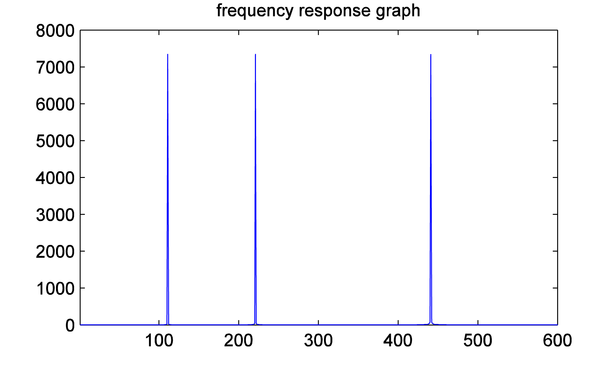
To plot the results of the fft function such that the values represent the magnitudes of the frequency components, we first apply the abs function to fftdata.
fftmag = abs(fftdata);
Let’s plot the frequency components to be sure we have what we think we have. For a sampling rate of sr on an array of sample values of size N, the Fourier transform returns the magnitudes of $$N/2$$ frequency components evenly spaced between 0 and sr/2 Hz. (We’ll explain this completely in Chapter 5.) Thus, we want to display frequencies between 0 and sr/2 on the horizontal axis, and only the first sr/2 values from the fftmag vector.
figure;
freqs = [0: (sr/2)-1];
plot(freqs, fftmag(1:sr/2));
[aside]If we would zoom in more closely at each of these spikes at frequencies 110, 220, and 440 Hz, we would see that they are not perfectly horizontal lines. The “imperfect” results of the FFT will be discussed later in the sections on FFT windows and windowing functions.[/aside] When you do this, you’ll see that all the frequency components are way over on the left side of the graph. Since we know our frequency components should be 110 Hz, 220 Hz, and 440 Hz, we might as well look at only the first, say, 600 frequency components so that we can see the results better. One way to zoom in on the frequency response graph is to use the zoom tool in the graph window, or you can reset the axis properties in the command window, as follows.
axis([0 600 0 8000]);
This yields the frequency response graph for our composite wave, which shows the three frequency components.
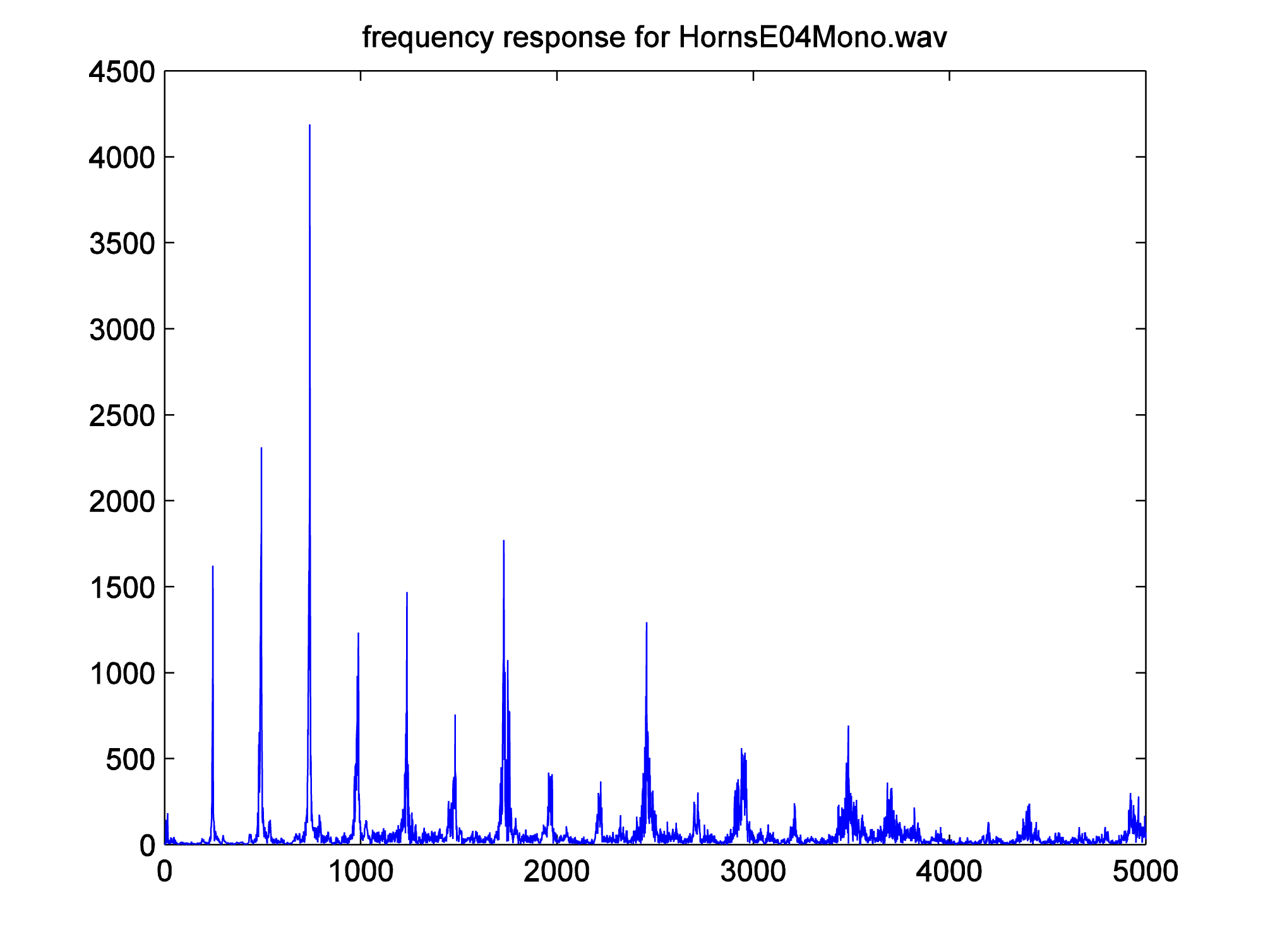
To get the phase response graph, we need to extract the phase information from the fftdata. This is done with the angle function. We leave that as an exercise. Let’s try the Fourier transform on a more complex sound wave – a sound file that we read in.
y = audioread('HornsE04Mono.wav');
As before, you can get the Fourier transform with the fft function.
fftdata = fft(y);
You can then get the magnitudes of the frequency components and generate a frequency response graph from this.
fftmag = abs(fftdata);
figure;
freqs = [0:(sr/2)-1];
plot(freqs, fftmag(1:sr/2));
axis([0 sr/2 0 4500]);
title('frequency response for HornsE04Mono.wav');
Let’s zoom in on frequencies up to 5000 Hz.
axis([0 5000 0 4500]);
The graph below is generated.
The inverse Fourier transform gives us back our original sound data in the time domain.
ynew = ifft(fftdata);
If you compare y with ynew, you’ll see that the inverse Fourier transform has recaptured the original sound data.