2.3.3 Modeling Sound in MATLAB

It’s easy to model and manipulate sound waves in MATLAB, a mathematical modeling program. If you learn just a few of MATLAB’s built-in functions, you can create sine waves that represent sounds of different frequencies, add them, plot the graphs, and listen to the resulting sounds. Working with sound in MATLAB helps you to understand the mathematics involved in digital audio processing. In this section, we’ll introduce you to the basic functions that you can use for your work in digital sound. This will get you started with MATLAB, and you can explore further on your own. If you aren’t able to use MATLAB, which is a commercial product, you can try substituting the freeware program Octave. We introduce you briefly to Octave in Section 2.3.5. In future chapters, we’ll limit our examples to MATLAB because it is widely used and has an extensive Signal Processing Toolbox that is extremely useful in sound processing. We suggest Octave as a free alternative that can accomplish some, but not all, of the examples in remaining chapters.

Before we begin working with MATLAB, let’s review the basic sine functions used to represent sound. In the equation y = Asin(2πfx + θ), frequency f is assumed to be measured in Hertz. An equivalent form of the sine function, and one that is often used, is expressed in terms of angular frequency, ω, measured in units of radians/s rather than Hertz. Since there are 2π radians in a cycle, and Hz is cycles/s, the relationship between frequency in Hertz and angular frequency in radians/s is as follows:

[equation caption=”Equation2.7″]Let f be the frequency of a sine wave in Hertz. Then the angular frequency, ω, in radians/s, is given by

$$!\omega =2\pi f$$

 

[/equation]

We can now give an alternative form for the sine function.

[equation caption=”Equation 2.8″]A single-frequency sound wave with angular frequency ω, amplitude , and A phase θ is represented by the sine function

 

$$!y=A\sin \left ( \omega t+\theta \right )$$

[/equation]

In our examples below, we show the frequency in Hertz, but you should be aware of these two equivalent forms of the sine function.   MATLAB’s sine function expects angular frequency in Hertz, so f must be multiplied by 2π.

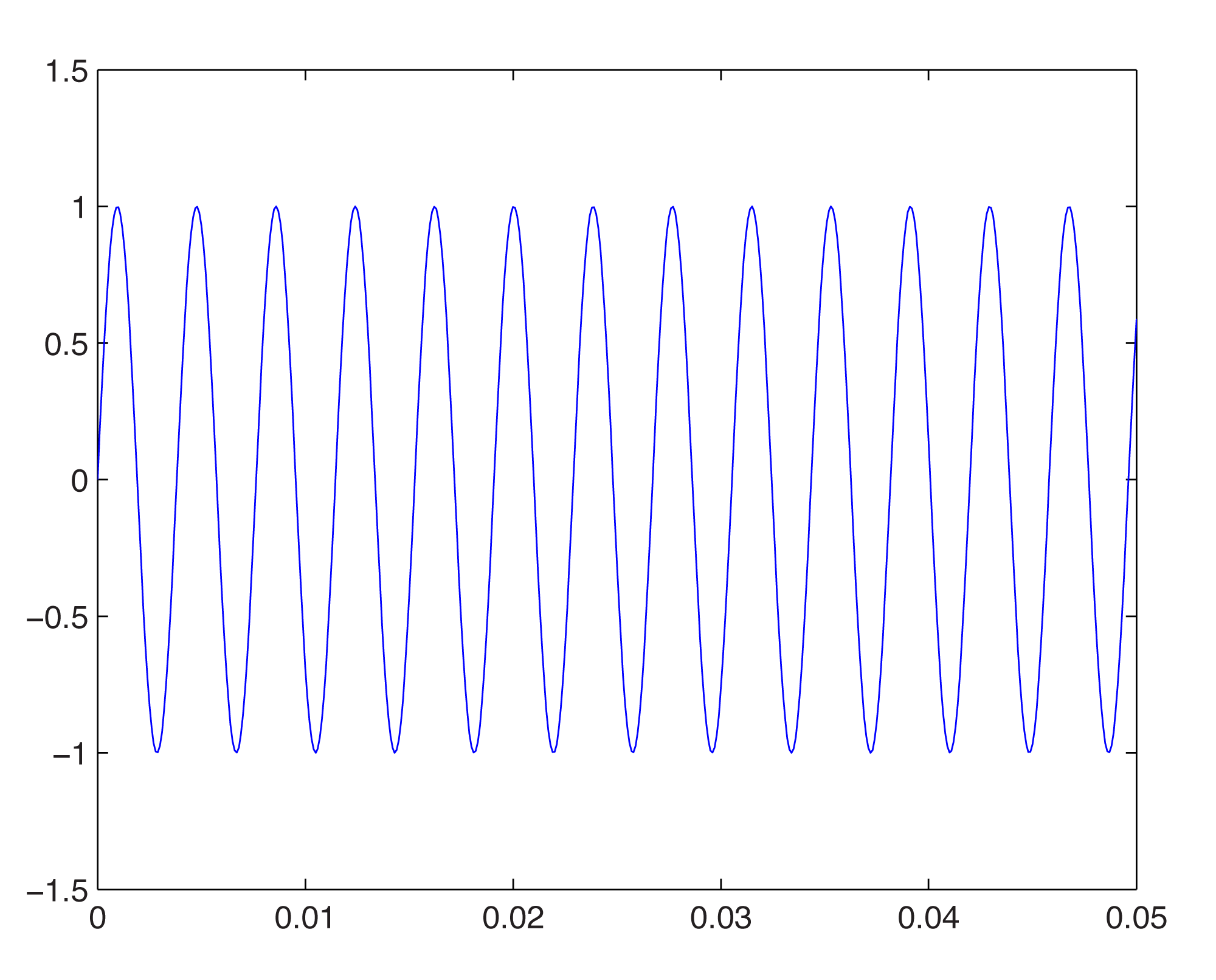
Now let’s look at how we can model sounds with sine functions in MATLAB. Middle C on a piano keyboard has a frequency of approximately 262 Hz. To create a sine wave in MATLAB at this frequency and plot the graph, we can use the fplot function as follows:

fplot('sin(262*2*pi*t)', [0, 0.05, -1.5, 1.5]);

The graph in Figure 2.30 pops open when you type in the above command and hit Enter. Notice that the function you want to graph is enclosed in single quotes. Also, notice that the constant π is represented as pi in MATLAB. The portion in square brackets indicates the limits of the horizontal and vertical axes. The horizontal axis goes from 0 to 0.05, and the vertical axis goes from –1.5 to 1.5.

If we want to change the amplitude of our sine wave, we can insert a value for A. If A > 1, we may have to alter the range of the vertical axis to accommodate the higher amplitude, as in

fplot('2*sin(262*2*pi*t)', [0, 0.05, -2.5, 2.5]);

After multiplying by A=2 in the statement above, the top of the sine wave goes to 2 rather than 1.

To change the phase of the sine wave, we add a value θ. Phase is essentially a relationship between two sine waves with the same frequency. When we add θ to the sine wave, we are creating a sine wave with a phase offset of θ compared to a sine wave with phase offset of 0. We can show this by graphing both sine waves on the same graph. To do so, we graph the first function with the command

fplot('2*sin(262*2*pi*t)', [0, 0.05, -2.5, 2.5]);

We then type

hold on

This will cause all future graphs to be drawn on the currently open figure. Thus, if we type

fplot('2*sin(262*2*pi*t+pi)', [0, 0.05, -2.5, 2.5]);

we have two phase-offset graphs on the same plot. In Figure 2.31, the 0-phase-offset sine wave is in red and the 180^o phase offset sine wave is in blue.

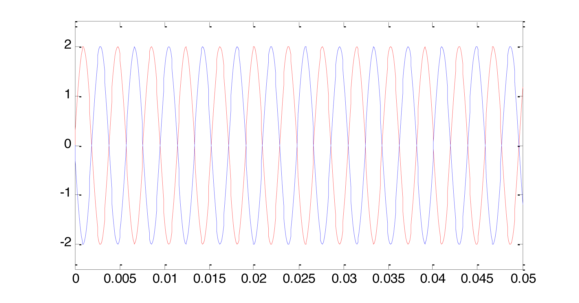
Notice that the offset is given in units of radians rather than degrees, 180^o being equal to radians.

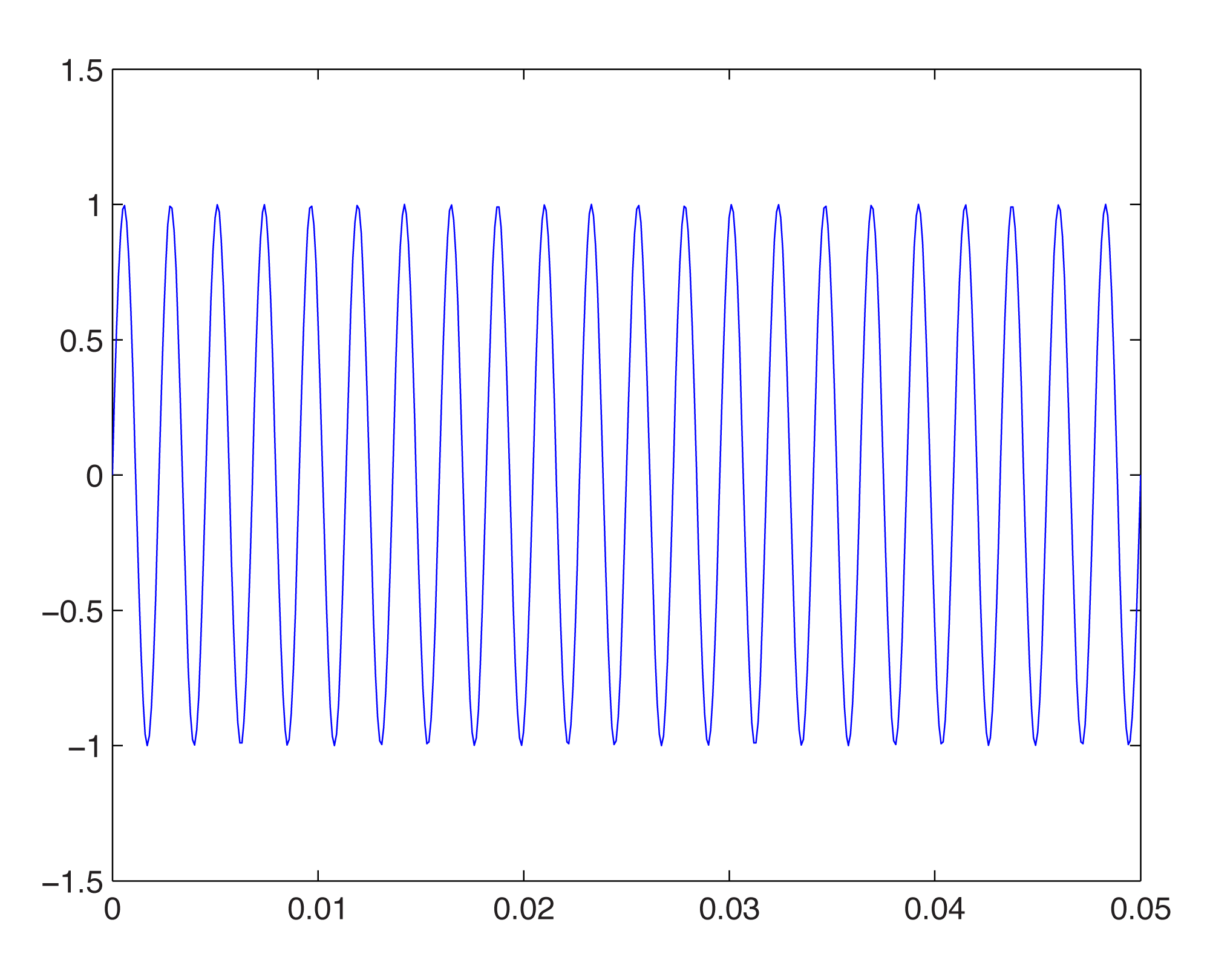
To change the frequency, we change ω. For example, changing ω to 440*2*pi gives us a graph of the note A above middle C on a keyboard.

fplot('sin(440*2*pi*t)', [0, 0.05, -1.5, 1.5]);

The above command gives this graph:

Then with

fplot('sin(262*2*pi*t)', [0, 0.05, -1.5, 1.5], 'red');

hold on

we get this figure:

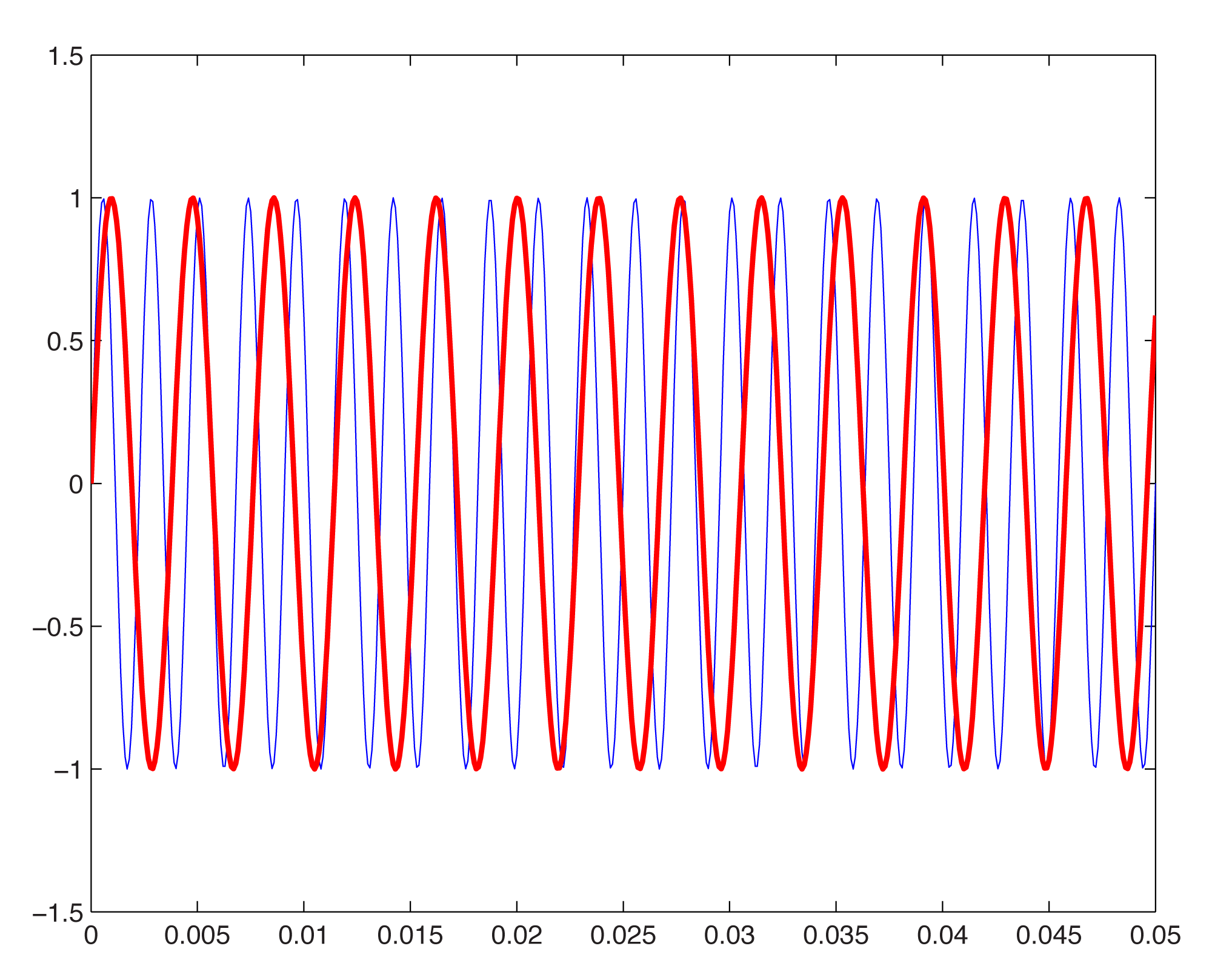
The 262 Hz sine wave in the graph is red to differentiate it from the blue 440 Hz wave.

The last parameter in the fplot function causes the graph to be plotted in red. Changing the color or line width also can be done by choosing Edit/Figure Properties on the figure, selecting the sine wave, and changing its properties.

We also can add sine waves to create more complex waves, as we did using Adobe Audition in Section 2.2.2. This is a simple matter of adding the functions and graphing the sum, as shown below.

figure

fplot('sin(262*2*pi*t)+sin(440*2*pi*t)', [0, 0.05, -2.5, 2.5]);

First, we type figure to open a new empty figure (so that our new graph is not overlaid on the currently open figure). We then graph the sum of the sine waves for the notes C and A. The result is this:

We’ve used the fplot function in these examples. This function makes it appear as if the graph of the sine function is continuous. Of course, MATLAB can’t really graph a continuous list of numbers, which would be infinite in length. The name MATLAB, in fact, is an abbreviation of “matrix laboratory.” MATLAB works with arrays and matrices. In Chapter 5, we’ll explain how sound is digitized such that a sound file is just an array of numbers. The plot function is the best one to use in MATLAB to graph these values. Here’s how this works.

First, you have to declare an array of values to use as input to a sine function. Let’s say that you want one second of digital audio at a sampling rate of 44,100 Hz (i.e., samples/s) (a standard sampling rate). Let’s set the values of variables for sampling rate sr and number of seconds s, just to remind you for future reference of the relationship between the two.

sr = 44100;
s = 1;

Now, to give yourself an array of time values across which you can evaluate the sine function, you do the following:

t = linspace(0,s, sr*s);

This creates an array of sr * s values evenly-spaced between and including the endpoints. Note that when you don’t put a semi-colon after a command, the result of the command is displayed on the screen. Thus, without a semi-colon above, you’d see the 44,100 values scroll in front of you.

To evaluate the sine function across these values, you type

y = sin(2*pi*262*t);

One statement in MATLAB can cause an operation to be done on every element of an array. In this example, y = sin(2*pi*262*t) takes the sine on each element of array t and stores the result in array y. To plot the sine wave, you type

plot(t,y);

Time is on the horizontal axis, between 0 and 1 second. Amplitude of the sound wave is on the vertical axis, scaled to values between -1 and 1. The graph is too dense for you to see the wave properly. There are three ways you can zoom in. One is by choosing Axes Properties from the graph’s Edit menu and then resetting the range of the horizontal axis. The second way is to type an axis command like the following:

axis([0 0.1 -2 2]);

This displays only the first 1/10 of a second on the horizontal axis, with a range of -2 to 2 on the vertical axis so you can see the shape of the wave better.

You can also ask for a plot of a subset of the points, as follows:

plot(t(1:1000),y(1:1000));

The above command plots only the first 1000 points from the sine function. Notice that the length of the two arrays must be the same for the plot function, and that numbers representing array indices must be positive integers. In general, if you have an array t of values and want to look at only the i^th to the j^th values, use t(i:j).

An advantage of generating an array of sample values from the sine function is that with that array, you actually can hear the sound. When you send the array to the wavplay or sound function, you can verify that you’ve generated one second’s worth of the frequency you wanted, middle C. You do this with

wavplay(y, sr);

(which works on Windows only) or, more generally,

sound(y, sr);

The first parameter is an array of sound samples. The second parameter is the sampling rate, which lets the system know how many samples to play per second.

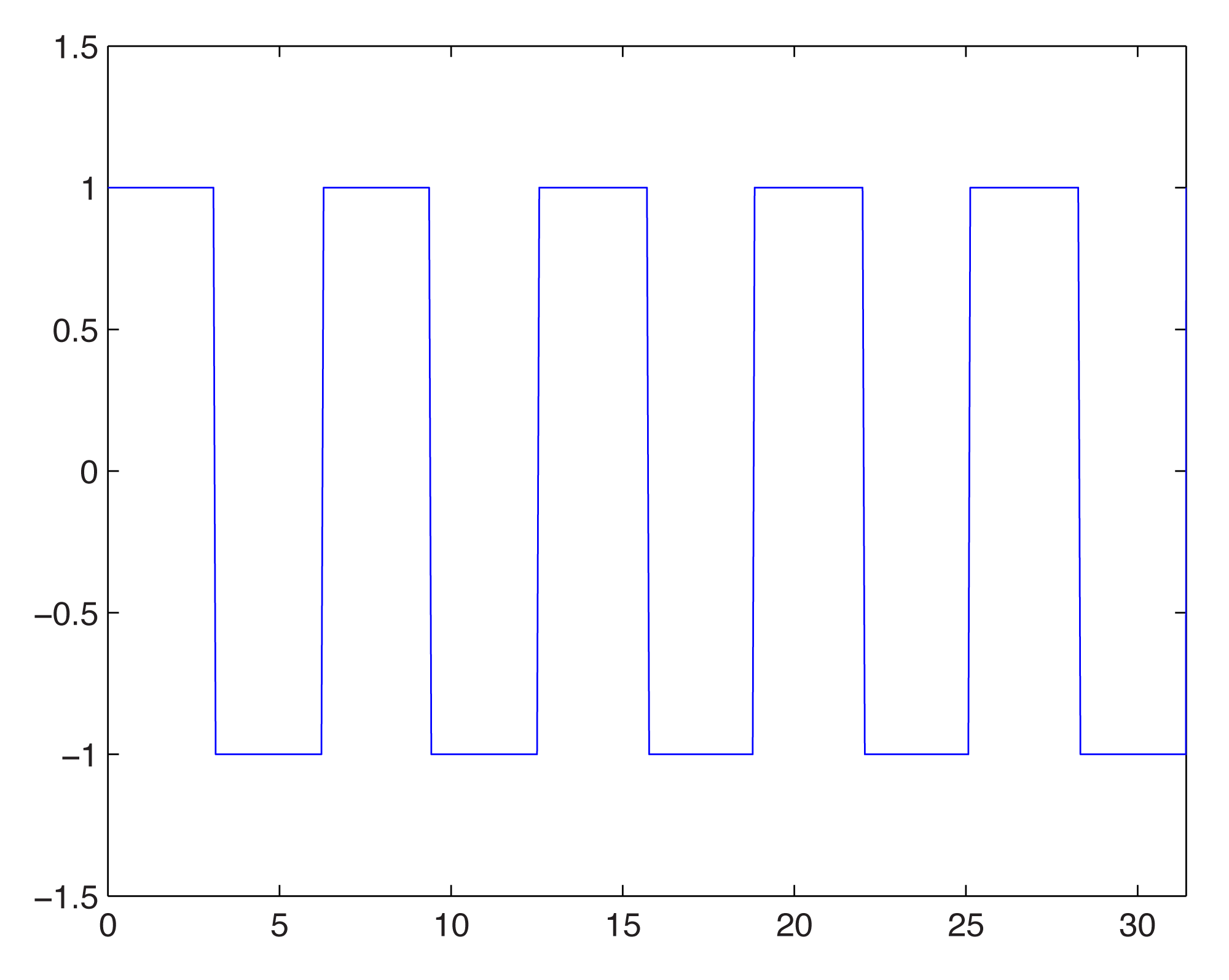
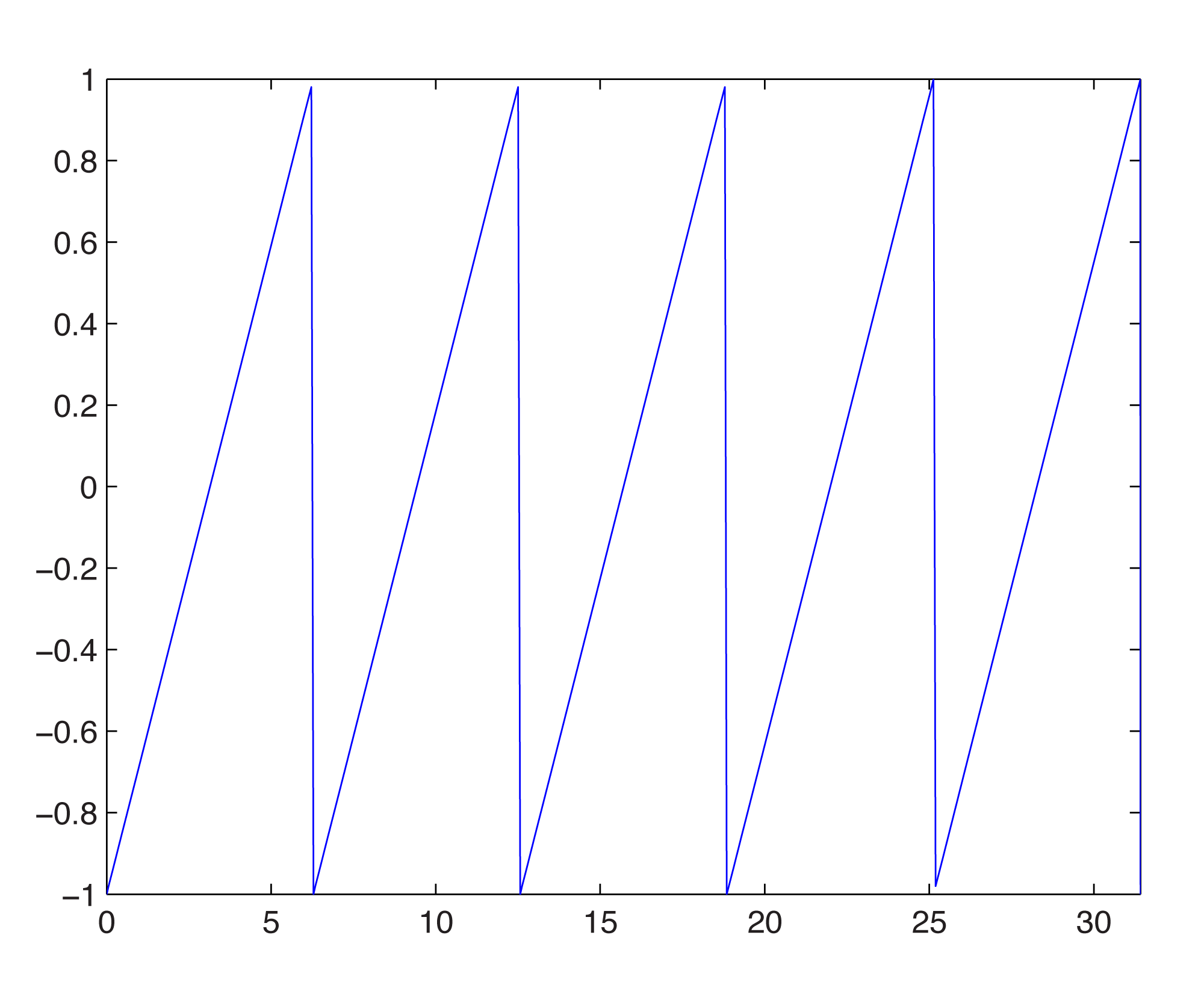
MATLAB has other built-in functions for generating waves of special shapes. We’ll go back to using fplot for these. For example, we can generate square, sawtooth, and triangular waves with the three commands given below:

fplot('square(t)',[0,10*pi,-1.5,1.5]);

fplot('sawtooth(t)',[0,10*pi]);

fplot('2*pulstran(t,[0:10],''tripuls'')-1',[0,10]);

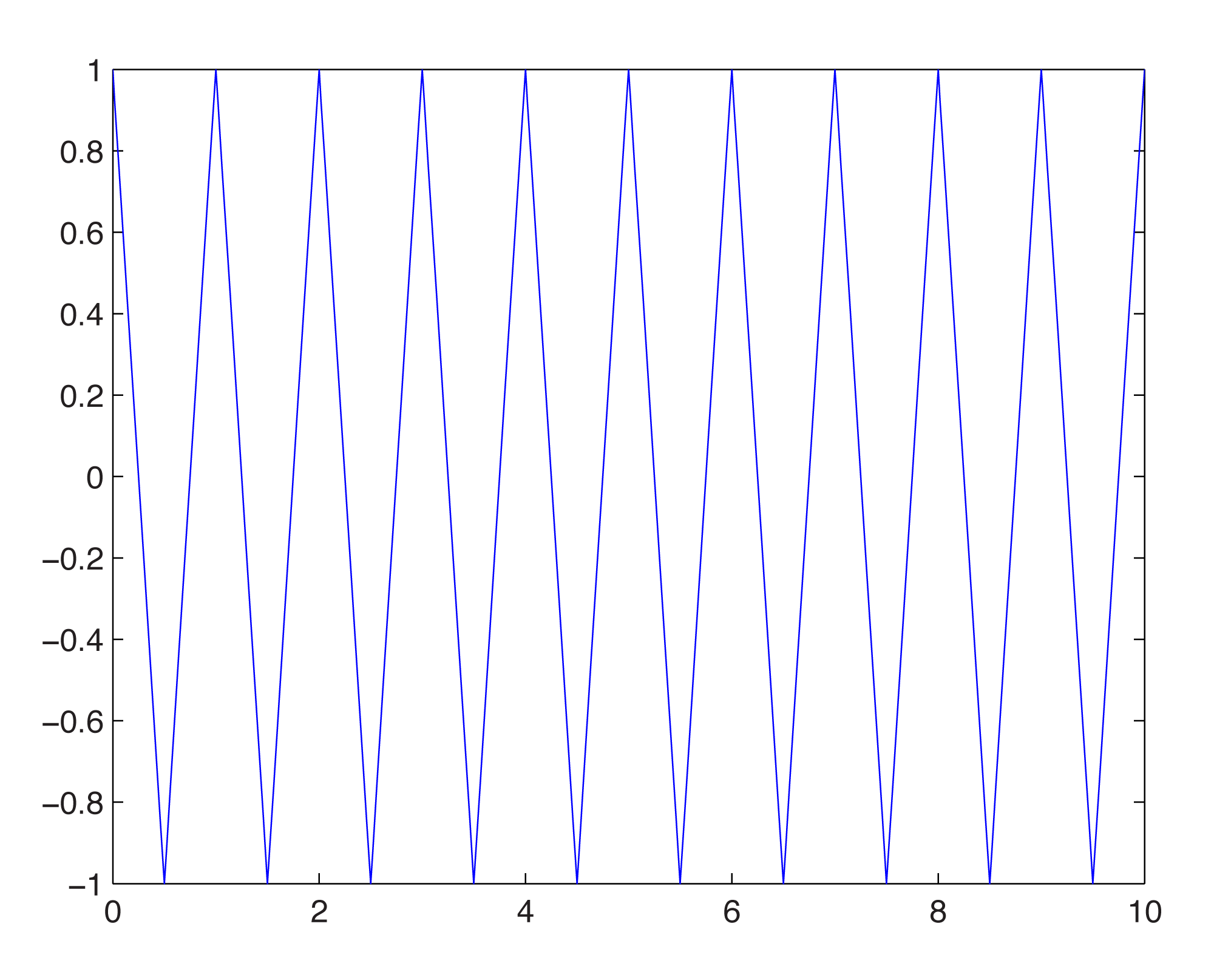
(Notice that the tripuls parameter is surrounded by two single quotes on each side.)

This section is intended only to introduce you to the basics of MATLAB for sound manipulation, and we leave it to you to investigate the above commands further. MATLAB has an extensive Help feature which gives you information on the built-in functions.

Each of the functions above can be created “from scratch” if you understand the nature of the non-sinusoidal waves. The ideal square wave is constructed from an infinite sum of odd-numbered harmonics of diminishing amplitude. More precisely, if f is the fundamental frequency of the non-sinusoidal wave to be created, then a square wave is constructed by the following infinite summation:

[equation caption=”Equation 2.9″]Let f be a fundamental frequency. Then a square wave created from this fundamental frequency is defined by the infinite summation

 

$$!\sum_{n=0}^{\infty }\frac{1}{\left ( 2n+1 \right )}\sin \left ( 2\pi \left ( 2n+1 \right )ft \right )$$

[/equation]

Of course, we can’t do an infinite summation in MATLAB, but we can observe how the graph of the function becomes increasingly square as we add more terms in the summation. To create the first four terms and plot the resulting sum, we can do

f1 = 'sin(2*pi*262*t) + sin(2*pi*262*3*t)/3 + sin(2*pi*262*5*t)/5 + sin(2*pi*262*7*t)/7';

fplot(f1, [0 0.01 -1 1]);

This gives the wave in Figure 2.38.

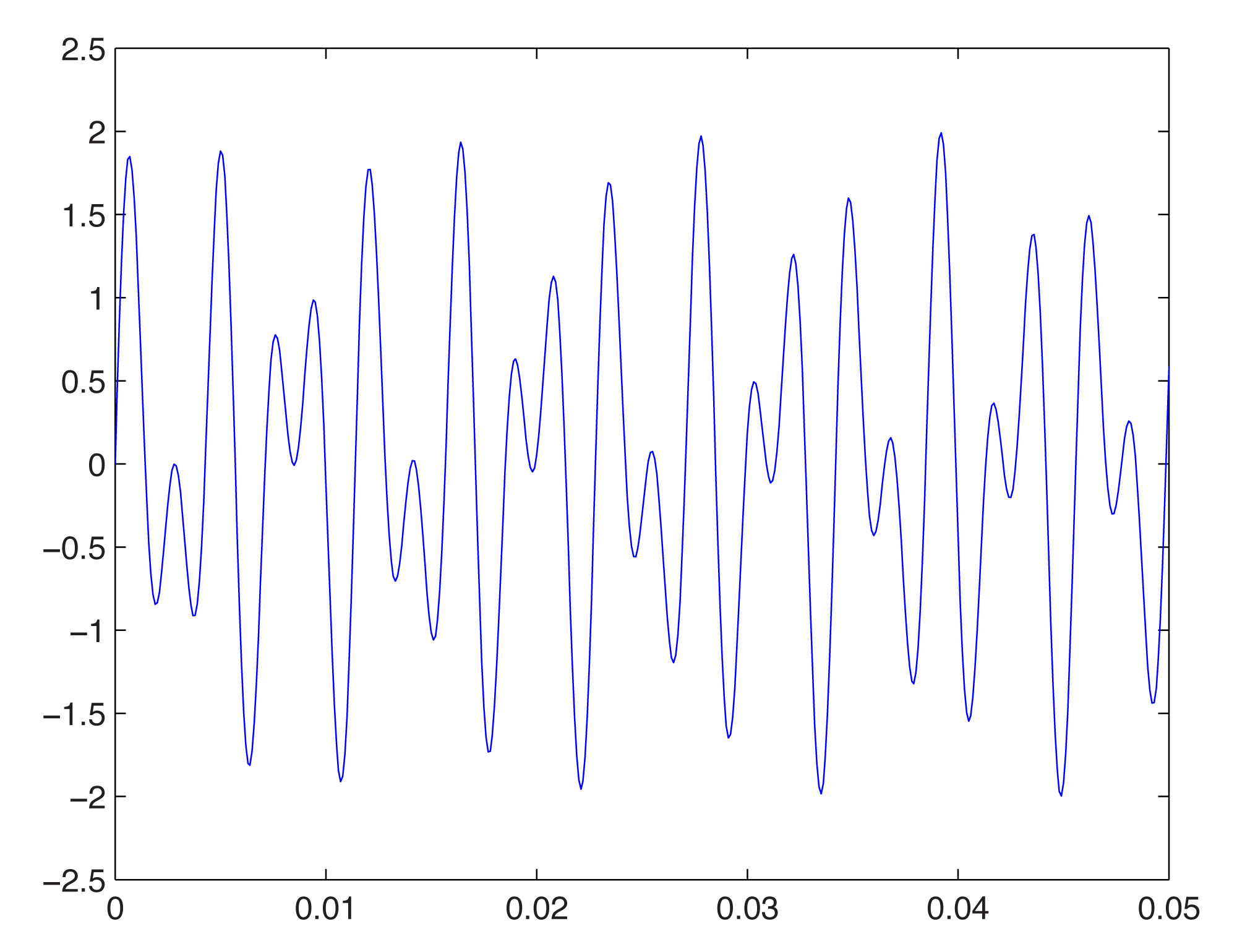
You can see that it is beginning to get square but has many ripples on the top. Adding four more terms gives further refinement to the square wave, as illustrated in Figure 2.39:

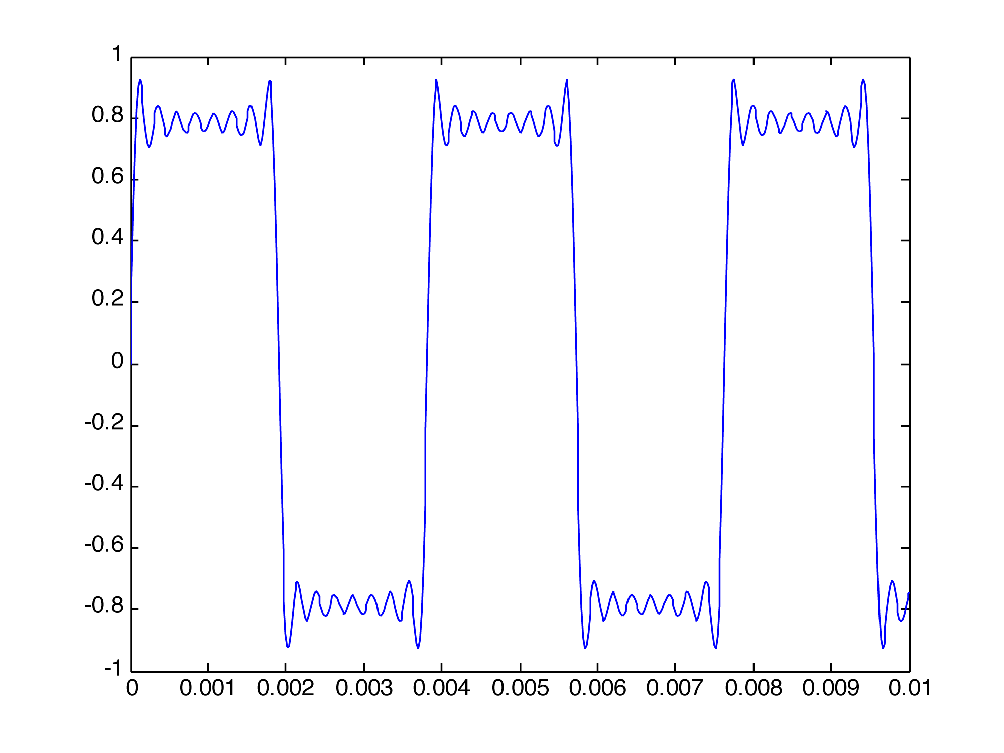
Creating the wave in this brute force manner is tedious. We can make it easier by using MATLAB’s sum function and its ability to do operations on entire arrays. For example, you can plot a 262 Hz square wave using 51 terms with the following MATLAB command:

fplot('sum(sin(2*pi*262*([1:2:101])*t)./([1:2:101]))',[0 0.005 -1 1])

The array notation [1:2:101] creates an array of 51 points spaced two units apart – in effect, including the odd harmonic frequencies in the summation and dividing by the odd number. The sum function adds up these frequency components. The function is graphed over the points 0 to 0.005 on the horizontal axis and –1 to 1 on the vertical axis. The ./ operation causes the division to be executed element by element across the two arrays.

The sawtooth wave is an infinite sum of all harmonic frequencies with diminishing amplitudes, as in the following equation:

[equation caption”Equation 2.10″]Let f be a fundamental frequency. Then a sawtooth wave created from this fundamental frequency is defined by the infinite summation

 

$$!\frac{2}{\pi }\sum_{n=1}^{\infty }\frac{\sin \left ( 2\pi n\, ft \right )}{n}$$

[/equation]

2/π is a scaling factor to ensure that the result of the summation is in the range of -1 to 1.

The sawtooth wave can be plotted by the following MATLAB command:

fplot('-sum((sin(2*pi*262*([1:100])*t)./([1:100])))',[0 0.005 -2 2])

The triangle wave is an infinite sum of odd-numbered harmonics that alternate in their signs, as follows:

[equation caption=”Equation 2.11″]Let f be a fundamental frequency. Then a triangle wave created from this fundamental frequency is defined by the infinite summation

 

$$!\frac{8}{\pi ^{2}}\sum_{n=0}^{\infty }\left ( \frac{sin\left ( 2\pi \left ( 4n+1 \right )ft \right )}{\left ( 4n+1 \right )^{2}} \right )-\left ( \frac{\sin \left ( 2\pi \left ( 4n+3 \right )ft \right )}{\left ( 4n+3 \right )^{2}} \right )$$

[/equation]

8/π^2 is a scaling factor to ensure that the result of the summation is in the range of -1 to 1.

We leave the creation of the triangle wave as a MATLAB exercise.

[wpfilebase tag=file id=51 tpl=supplement /]

If you actually want to hear one of these waves, you can generate the array of audio samples with

s = 1;

sr = 44100;

t = linspace(0, s, sr*s);

y = sawtooth(262*2*pi*t);

and then play the wave with

sound(y, sr);

It’s informative to create and listen to square, sawtooth, and triangle waves of various amplitudes and frequencies. This gives you some insight into how these waves can be used in sound synthesizers to mimic the sounds of various instruments. We’ll cover this in more detail in Chapter 6.

In this chapter, all our MATLAB examples are done by means of expressions that are evaluated directly from MATLAB’s command line. Another way to approach the problems is to write programs in MATLAB’s scripting language. We leave it to the reader to explore MATLAB script programming, and we’ll have examples in later chapters.