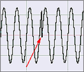
In addition to choosing the FFT window size, audio processing programs often let you choose from a number of windowing functions. The purpose of an FFT windowing function is to smooth out the discontinuities that result from applying the FFT to segments (i.e., windows) of audio data. A simplifying assumption for the FFT is that each windowed segment of audio data contains an integral number of cycles, this cycle repeating throughout the audio. This, of course, is not generally the case. If it were the case – that is, if the window ended exactly where the cycle ended – then the end of the cycle would be at exactly the same amplitude as the beginning. The beginning and end would “match up.” The actual discontinuity between the end of a window and its beginning is interpreted by the FFT as a jump from one level to another, as shown in Figure 2.51. (In this figure, we’ve cut and pasted a portion from the beginning of the window to its end to show that the ends don’t match up.)
In the output of the FFT, the discontinuity between the ends and the beginnings of the windows manifests itself as frequency components that don’t really exist in audio – called spurious frequencies, or spectral leakage. You can see the spectral leakage Figure 2.41. Although the audio signal actually contains only one frequency at 880 Hz, the frequency analysis view indicates that there is a small amount of other frequencies across the audible spectrum.
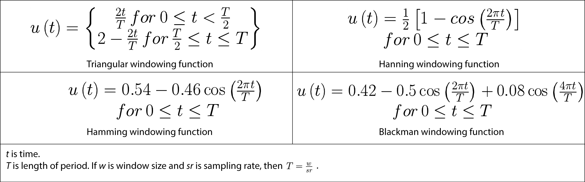
In order to smooth over this discontinuity and thereby reduce the amount of spectral leakage, the windowing functions effectively taper the ends of the segments to 0 so that they connect from beginning to end. The drop-down menu to the left of the FFT size menu in Audition is where you choose the windowing function. In Figure 2.50, the Hanning function is chosen. Four commonly-used windowing functions are given in the table below.
Windowing functions are easy to apply. The segment of audio data being transformed is simply multiplied by the windowing function before the transform is applied. In MATLAB, you can accomplish this with vector multiplication, as shown in the commands below.
y = audioread('HornsE04Mono.wav');
sr = 44100; %sampling rate
w = 2048; %window size
T = w/sr; %period
% t is an array of times at which the hamming function is evaluated
t = linspace(0, 1, 44100);
twindow = t(1:2048); %first 2048 elements of t
% Create the values for the hamming function, stored in vector called hamming
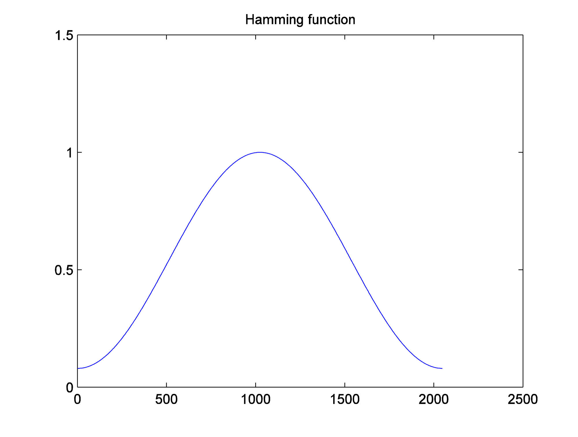
hamming = 0.54 - 0.46 * cos((2 * pi * twindow)/T);
plot(hamming);
title('Hamming');
The Hamming function is shown in
yshort = y(1:2048); %first 2048 samples from sound file
%Multiply the audio values in the window by the Hamming function values,
% using element by element multiplication with .*.
% first convert hamming from a column vector to a row vector
ywindowed = hamming .* yshort;
figure;
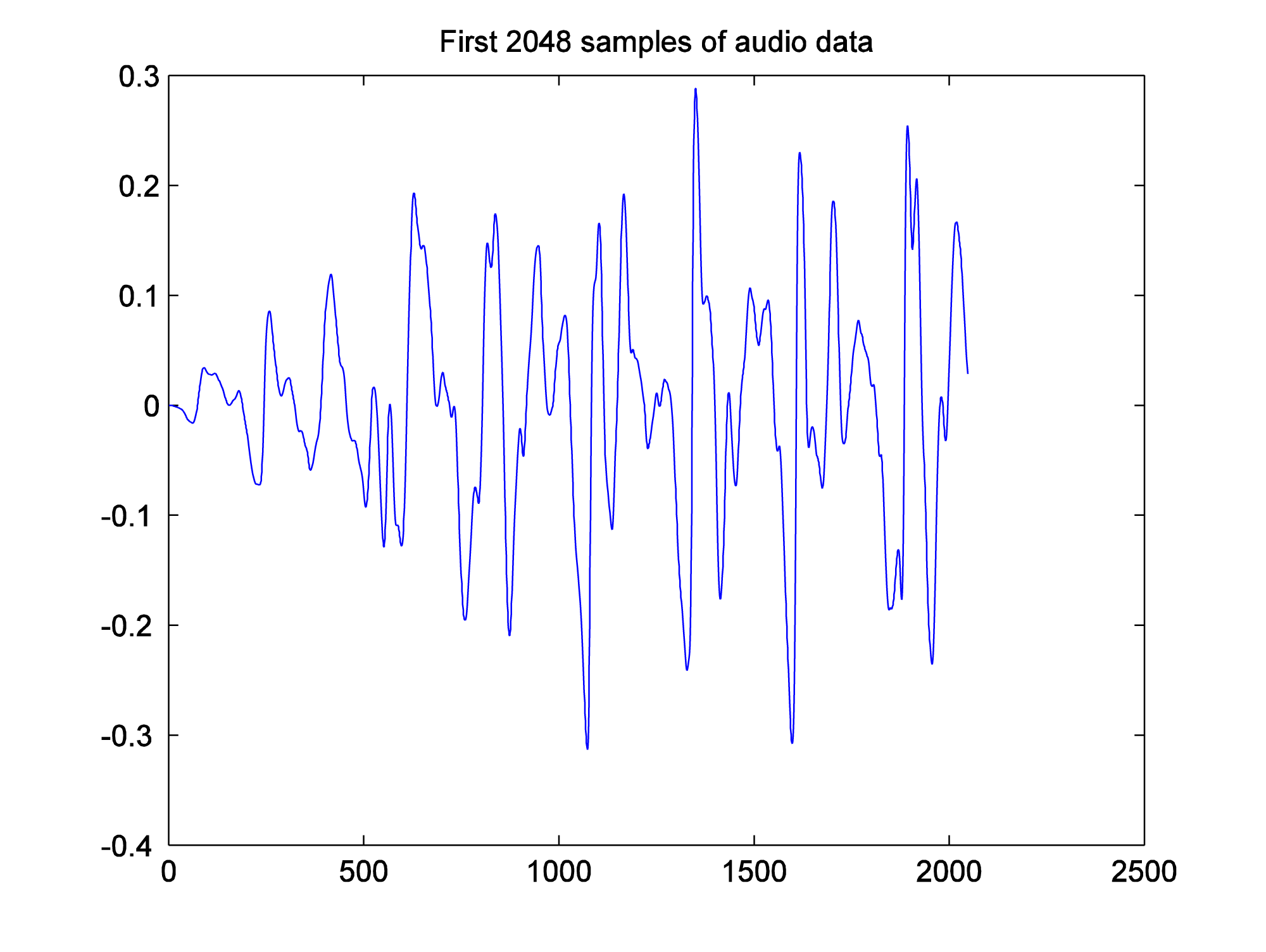
plot(yshort);
title('First 2048 samples of audio data');
figure;
plot(ywindowed);
title('First 2048 samples of audio data, tapered by windowing function');
Before the Hamming function is applied, the first 2048 samples of audio data look like this:
After the Hamming function is applied, the audio data look like this:
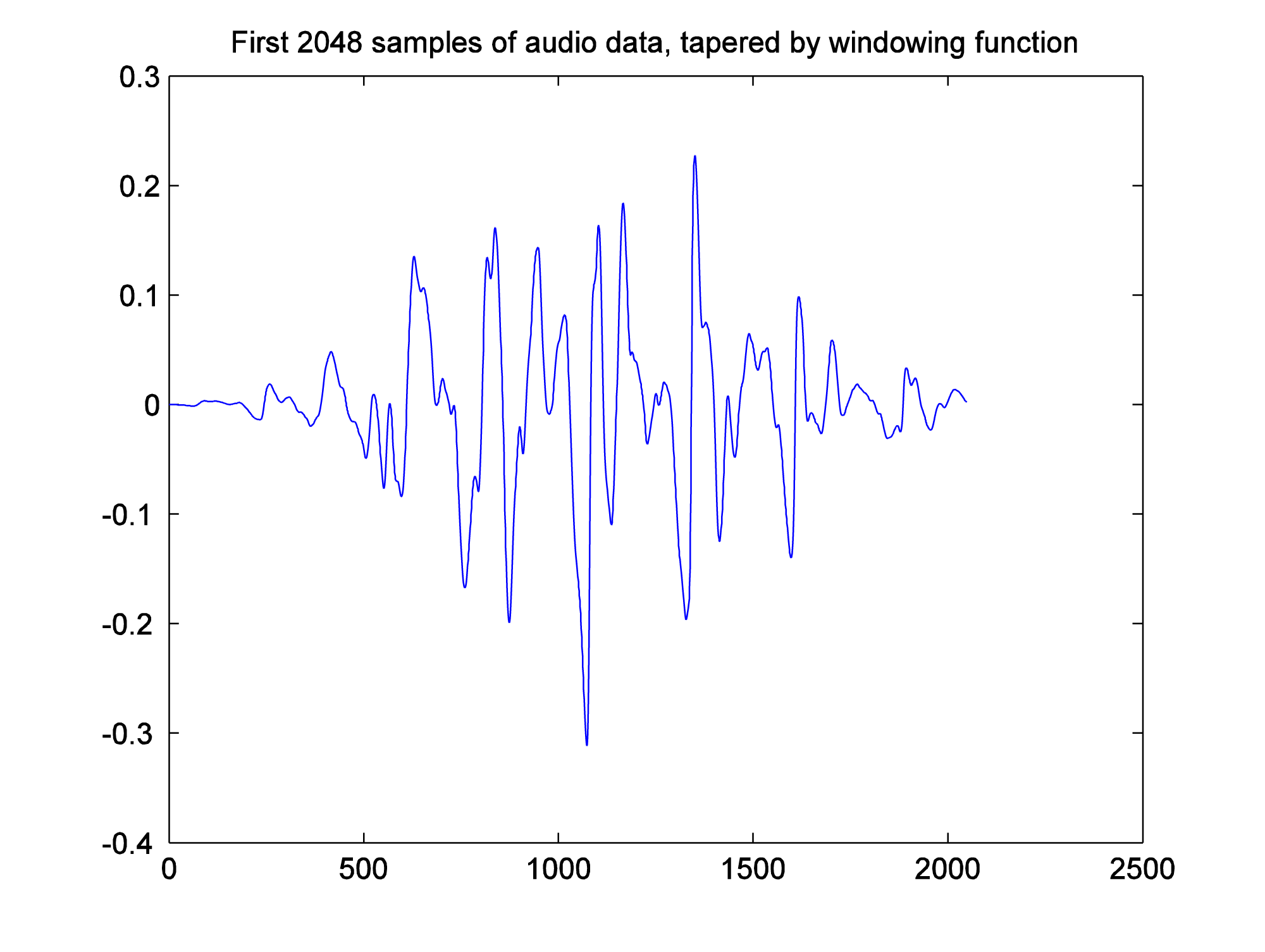
Notice that the ends of the segment are tapered toward 0.
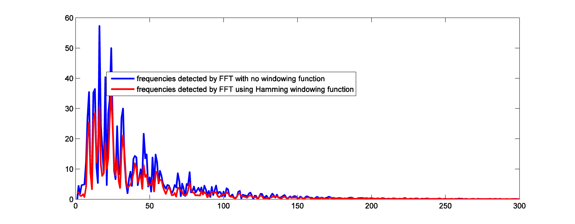
Figure 2.56 compares the FFT results with no windowing function vs. with the Hamming windowing function applied. The windowing function eliminates some of the high frequency components that are caused by spectral leakage.
figure
plot(abs(fft(yshort)));
axis([0 300 0 60]);
hold on;
plot(abs(fft(ywindowed)),'r');
[wpfilebase tag=file id=126 tpl=supplement /]
[separator top=”1″ bottom=”0″ style=”none”]