We showed in the previous section how we can add frequency components to create a complex sound wave. The reverse of the sound synthesis process is sound analysis, which is the determination of the frequency components in a complex sound wave. In the 1800s, Joseph Fourier developed the mathematics that forms the basis of frequency analysis. He proved that any periodic sinusoidal function, regardless of its complexity, can be formulated as a sum of frequency components. These frequency components consist of a fundamental frequency and the harmonic frequencies related to this fundamental. Fourier’s theorem says that no matter how complex a sound is, it’s possible to break it down into its component frequencies – that is, to determine the different frequencies that are in that sound, and how much of each frequency component there is.
[aside]”Frequency response” has a number of related usages in the realm of sound. It can refer to a graph showing the relative magnitudes of audible frequencies in a given sound. With regard to an audio filter, the frequency response shows how a filter boosts or attenuates the frequencies in the sound to which it is applied. With regard to loudspeakers, the frequency response is the way in which the loudspeakers boost or attenuate the audible frequencies. With regard to a microphone, the frequency response is the microphone’s sensitivity to frequencies over the audible spectrum.[/aside]
Fourier analysis begins with the fundamental frequency of the sound – the frequency of the longest repeated pattern of the sound. Then all the remaining frequency components that can be yielded by Fourier analysis – i.e., the harmonic frequencies – are integer multiples of the fundamental frequency. By “integer multiple” we mean that if the fundamental frequency is $$f_0$$ , then each harmonic frequency $$f_n$$ is equal to for some non-negative integer $$(n+1)f_0$$.
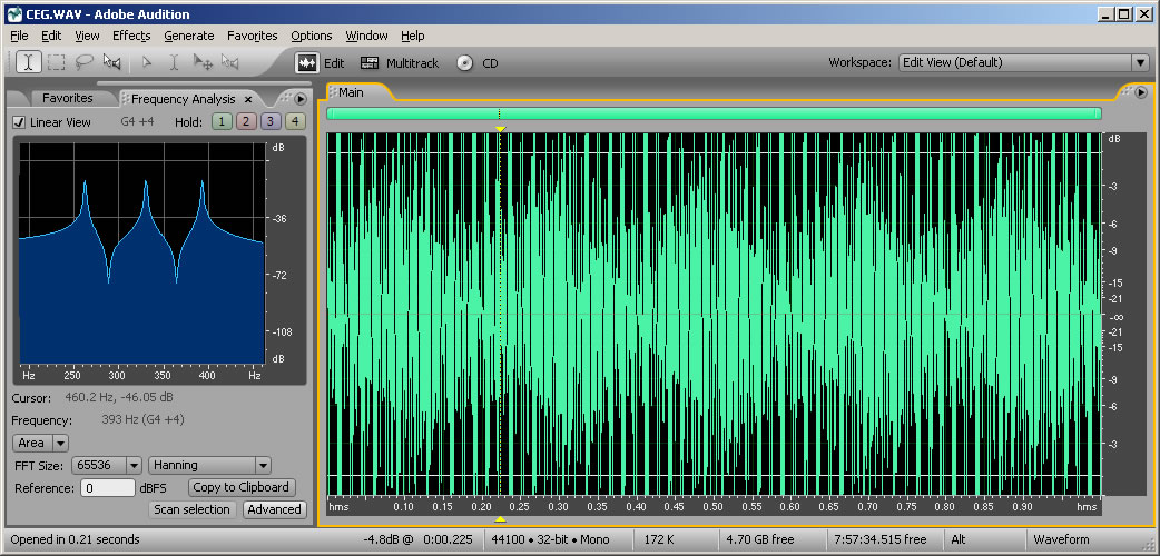
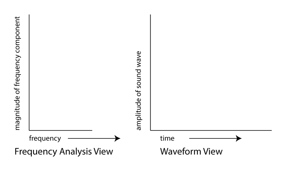
The Fourier transform is a mathematical operation used in digital filters and frequency analysis software to determine the frequency components of a sound. Figure 2.17 shows Adobe Audition’s waveform view and a frequency analysis view for a sound with frequency components at 262 Hz, 330 Hz, and 393 Hz. The frequency analysis view is to the left of the waveform view. The graph in the frequency analysis view is called a frequency response graph or simply a frequency response. The waveform view has time on the x-axis and amplitude on the y-axis. The frequency analysis view has frequency on the x-axis and the magnitude of the frequency component on the y-axis. (See Figure 2.18.) In the frequency analysis view in Figure 2.17, we zoomed in on the portion of the x-axis between about 100 and 500 Hz to show that there are three spikes there, at approximately the positions of the three frequency components. You might expect that there would be three perfect vertical lines at 262, 330, and 393 Hz, but this is because digitizing and transforming sound introduces some error. Still, the Fourier transform is accurate enough to be the basis for filters and special effects with sounds.
In the example just discussed, the frequencies that are combined in the composite sound never change. This is because of the way we constructed the sound, with three single-frequency waves that are held for one second. This sound, overall, is periodic because the pattern created from adding these three component frequencies is repeated over time, as you can see in the bottom of Figure 2.14.
Natural sounds, however, generally change in their frequency components as time passes. Consider something as simple as the word “information.” When you say “information,” your voice produces numerous frequency components, and these change over time. Figure 2.19 shows a recording and frequency analysis of the spoken word “information.”
When you look at the frequency analysis view, don’t be confused into thinking that the x-axis is time. The frequencies being analyzed are those that are present in the sound around the point in time marked by the yellow line.

In music and other sounds, pitches – i.e., frequencies – change as time passes. Natural sounds are not periodic in the way that a one-chord sound is. The frequency components in the first second of such sounds are different from the frequency components in the next second. The upshot of this fact is that for complex non-periodic sounds, you have to analyze frequencies over a specified time period, called a window. When you ask your sound analysis software to provide a frequency analysis, you have to set the window size. The window size in Adobe Audition’s frequency analysis view is called “FFT size.” In the examples above, the window size is set to 65536, indicating that the analysis is done over a span of 65,536 audio samples. The meaning of this window size is explained in more detail in Chapter 7. What is important to know at this point is that there’s a tradeoff between choosing a large window and a small one. A larger window gives higher resolution across the frequency spectrum – breaking down the spectrum into smaller bands – but the disadvantage is that it “blurs” its analysis of the constantly changing frequencies across a larger span of time. A smaller window focuses on what the frequency components are in a more precise, short frame of time, but it doesn’t yield as many frequency bands in its analysis.